Embedding a neuron model in a network model¶

ISF defines network connectivity between presynaptic cells and a postsynaptic neuron model in terms of two files:

The .syn file defines the location of synapses onto a postsynaptic morphology, including the type of the corresponding presynaptic cell
The .con file defines for each synapse the corresponding ID, and the presynaptic cell ID. Each presynaptic cell may have one or more synapses with the postsynaptic neuron.

ISF provides a way to generate this connectivity data based on an empirically quantified dense anatomical model, as shown in this section

Info

Some model systems may not have the necessary data available for this pipeline, or infer connectivity from anatomical models in different ways. You can still use ISF for those model systems. In these cases, we highly recommend to generate synapse locations on the postsynaptic morphology in whichever form is most suitable to your model system, and convert the connectivity specification to the ISF file formats: .syn and .con.

Warning

If you decide to use your own methods for inferring synapse locations onto the neuron model morphology, it may be necessary to use methods based on empirically verified dense anatomical models. Otherwise, simulation results may not be empirically consistent, or predictions based on these results may not successfully generalize to in vivo conditions.

The .syn file ¶

.syn files define the location of synapses onto a postsynaptic morphology. As such, they are only valid for one specific morphology.

Let’s have a look at what exactly a .syn file looks like.

[1]:

from getting_started import example_data_dir
from pathlib import Path
example_embedding_dir = Path(example_data_dir) / "anatomical_constraints" / "example_embedding_86_C2_center"

[2]:

example_syn_fn = [e for e in example_embedding_dir.glob("*.syn")][0]
with open(example_syn_fn) as input_file:
    head = [next(input_file) for _ in range(10)]
print("".join(head))

# Synapse distribution file
# corresponding to cell: 86_C2_center
# Type - section - section.x

VPM_E1  112     0.138046479525
VPM_E1  130     0.305058053119
VPM_E1  130     0.190509288017
VPM_E1  9       0.368760777084
VPM_E1  110     0.0
VPM_E1  11      0.120662910562

The .syn file consists of a three-line header, a blank line, and then the connectivity data.

The header of the .syn file defines what the file is, to which morphology file this .syn file belongs, and the names of the three columns:

Type: the type of the presynaptic cell that connects with this synapse
section: the section number of the postsynaptic morphology where this synapse connects
section.x: the relative coordinate on this section where this synapse connects

Each line corresponds to a single synapse. Each synapse has an ID that equals the index of this line, starting at 0.

A single .syn file uniquely defines, for one morphology, where each synapse is located on the dendritic tree, and what the corresponding presynaptic cell type is for each synapse.

The .con file ¶

A .con file defines to which presynaptic cell each synapse belongs.

[3]:

example_con_fn = [e for e in example_embedding_dir.glob("*.con")][0]
with open(example_con_fn) as input_file:
    head = [next(input_file) for _ in range(10)]
print("".join(head))

# Anatomical connectivity realization file; only valid with synapse realization:
# example_embedding_86_C2_center.syn
# Type - cell ID - synapse ID

L6cc_A3 0       0
L6cc_A3 1       1
L6cc_A3 2       2
L6cc_A3 3       3
L6cc_A3 4       4
L6cc_A3 4       5

We see that the .con file again describes a three-line header. This time, it backlinks to a .syn file and again defines three columns:

Type: the type of the presynaptic cell this synapse belongs to. It is added for redundancy, so that this file is interpretable in isolation.
cell ID: the ID of the presynaptic cell this synaps belongs to. This is not necessarily the same as the ID of the synapse. The same cell can make multiple synaptic connections with a postsynaptic neuron. These IDs are only the same if each synapse belongs to a unique presynaptic cell.
synapse ID: the ID of this synapse. This corresponds to the row index in a .syn file. This also explains why the corresponding .syn file is mentioned in the header.

.con files provide some redundant information when combined with .syn files. This is simply to keep these files interpretable and informative when viewed in isolation.

The network parameters ¶

Network parameters define all parameters that relate to a network; both connectivity (this tutorial) and activity (next tutorial). The next tutorial will build a fully functional network parameters that can be used for simulations of network-embedded neuron models.

For the sake of completeness, we already show here how to build one containing just connectivity info.

[4]:

from singlecell_input_mapper.network_param_builder import NetworkParamBuilder

netp = NetworkParamBuilder().add_network_embedding(
    syn_fn = example_syn_fn,
    con_fn = example_con_fn,
    join="right"  # right-join the incoming connectivity data to the network parameters (default is left)
)

netp.network_parameters.as_dict()

Warning: no DISPLAY environment variable.
--No graphics will be displayed.

[4]:

{'info': {'date': '2026-04-23', 'name': 'meulemeester'},
 'network': {'L1_B1': {'cellNr': 8,
   'synapses': {'distributionFile': PosixPath('/gpfs/soma_fs/scratch/meulemeester/project_src/in_silico_framework/getting_started/example_data/anatomical_constraints/example_embedding_86_C2_center/example_embedding_86_C2_center.syn'),
    'connectionFile': PosixPath('/gpfs/soma_fs/scratch/meulemeester/project_src/in_silico_framework/getting_started/example_data/anatomical_constraints/example_embedding_86_C2_center/example_embedding_86_C2_center.con')}},
  'L1_B2': {'cellNr': 10,
   'synapses': {'distributionFile': PosixPath('/gpfs/soma_fs/scratch/meulemeester/project_src/in_silico_framework/getting_started/example_data/anatomical_constraints/example_embedding_86_C2_center/example_embedding_86_C2_center.syn'),
    'connectionFile': PosixPath('/gpfs/soma_fs/scratch/meulemeester/project_src/in_silico_framework/getting_started/example_data/anatomical_constraints/example_embedding_86_C2_center/example_embedding_86_C2_center.con')}},
  'L1_B3': {'cellNr': 3,
   'synapses': {'distributionFile': PosixPath('/gpfs/soma_fs/scratch/meulemeester/project_src/in_silico_framework/getting_started/example_data/anatomical_constraints/example_embedding_86_C2_center/example_embedding_86_C2_center.syn'),
    'connectionFile': PosixPath('/gpfs/soma_fs/scratch/meulemeester/project_src/in_silico_framework/getting_started/example_data/anatomical_constraints/example_embedding_86_C2_center/example_embedding_86_C2_center.con')}},
  'L1_Beta': {'cellNr': 2,
   'synapses': {'distributionFile': PosixPath('/gpfs/soma_fs/scratch/meulemeester/project_src/in_silico_framework/getting_started/example_data/anatomical_constraints/example_embedding_86_C2_center/example_embedding_86_C2_center.syn'),
    'connectionFile': PosixPath('/gpfs/soma_fs/scratch/meulemeester/project_src/in_silico_framework/getting_started/example_data/anatomical_constraints/example_embedding_86_C2_center/example_embedding_86_C2_center.con')}},
  'L1_C1': {'cellNr': 15,
   'synapses': {'distributionFile': PosixPath('/gpfs/soma_fs/scratch/meulemeester/project_src/in_silico_framework/getting_started/example_data/anatomical_constraints/example_embedding_86_C2_center/example_embedding_86_C2_center.syn'),
    'connectionFile': PosixPath('/gpfs/soma_fs/scratch/meulemeester/project_src/in_silico_framework/getting_started/example_data/anatomical_constraints/example_embedding_86_C2_center/example_embedding_86_C2_center.con')}},
  'L1_C2': {'cellNr': 43,
   'synapses': {'distributionFile': PosixPath('/gpfs/soma_fs/scratch/meulemeester/project_src/in_silico_framework/getting_started/example_data/anatomical_constraints/example_embedding_86_C2_center/example_embedding_86_C2_center.syn'),
    'connectionFile': PosixPath('/gpfs/soma_fs/scratch/meulemeester/project_src/in_silico_framework/getting_started/example_data/anatomical_constraints/example_embedding_86_C2_center/example_embedding_86_C2_center.con')}},
  'L1_C3': {'cellNr': 15,
   'synapses': {'distributionFile': PosixPath('/gpfs/soma_fs/scratch/meulemeester/project_src/in_silico_framework/getting_started/example_data/anatomical_constraints/example_embedding_86_C2_center/example_embedding_86_C2_center.syn'),
    'connectionFile': PosixPath('/gpfs/soma_fs/scratch/meulemeester/project_src/in_silico_framework/getting_started/example_data/anatomical_constraints/example_embedding_86_C2_center/example_embedding_86_C2_center.con')}},
  'L1_D1': {'cellNr': 6,
   'synapses': {'distributionFile': PosixPath('/gpfs/soma_fs/scratch/meulemeester/project_src/in_silico_framework/getting_started/example_data/anatomical_constraints/example_embedding_86_C2_center/example_embedding_86_C2_center.syn'),
    'connectionFile': PosixPath('/gpfs/soma_fs/scratch/meulemeester/project_src/in_silico_framework/getting_started/example_data/anatomical_constraints/example_embedding_86_C2_center/example_embedding_86_C2_center.con')}},
  'L1_D2': {'cellNr': 26,
   'synapses': {'distributionFile': PosixPath('/gpfs/soma_fs/scratch/meulemeester/project_src/in_silico_framework/getting_started/example_data/anatomical_constraints/example_embedding_86_C2_center/example_embedding_86_C2_center.syn'),
    'connectionFile': PosixPath('/gpfs/soma_fs/scratch/meulemeester/project_src/in_silico_framework/getting_started/example_data/anatomical_constraints/example_embedding_86_C2_center/example_embedding_86_C2_center.con')}},
  'L1_D3': {'cellNr': 8,
   'synapses': {'distributionFile': PosixPath('/gpfs/soma_fs/scratch/meulemeester/project_src/in_silico_framework/getting_started/example_data/anatomical_constraints/example_embedding_86_C2_center/example_embedding_86_C2_center.syn'),
    'connectionFile': PosixPath('/gpfs/soma_fs/scratch/meulemeester/project_src/in_silico_framework/getting_started/example_data/anatomical_constraints/example_embedding_86_C2_center/example_embedding_86_C2_center.con')}},
  'L1_E2': {'cellNr': 3,
   'synapses': {'distributionFile': PosixPath('/gpfs/soma_fs/scratch/meulemeester/project_src/in_silico_framework/getting_started/example_data/anatomical_constraints/example_embedding_86_C2_center/example_embedding_86_C2_center.syn'),
    'connectionFile': PosixPath('/gpfs/soma_fs/scratch/meulemeester/project_src/in_silico_framework/getting_started/example_data/anatomical_constraints/example_embedding_86_C2_center/example_embedding_86_C2_center.con')}},
  'L23Trans_B1': {'cellNr': 1,
   'synapses': {'distributionFile': PosixPath('/gpfs/soma_fs/scratch/meulemeester/project_src/in_silico_framework/getting_started/example_data/anatomical_constraints/example_embedding_86_C2_center/example_embedding_86_C2_center.syn'),
    'connectionFile': PosixPath('/gpfs/soma_fs/scratch/meulemeester/project_src/in_silico_framework/getting_started/example_data/anatomical_constraints/example_embedding_86_C2_center/example_embedding_86_C2_center.con')}},
  'L23Trans_B2': {'cellNr': 7,
   'synapses': {'distributionFile': PosixPath('/gpfs/soma_fs/scratch/meulemeester/project_src/in_silico_framework/getting_started/example_data/anatomical_constraints/example_embedding_86_C2_center/example_embedding_86_C2_center.syn'),
    'connectionFile': PosixPath('/gpfs/soma_fs/scratch/meulemeester/project_src/in_silico_framework/getting_started/example_data/anatomical_constraints/example_embedding_86_C2_center/example_embedding_86_C2_center.con')}},
  'L23Trans_B3': {'cellNr': 2,
   'synapses': {'distributionFile': PosixPath('/gpfs/soma_fs/scratch/meulemeester/project_src/in_silico_framework/getting_started/example_data/anatomical_constraints/example_embedding_86_C2_center/example_embedding_86_C2_center.syn'),
    'connectionFile': PosixPath('/gpfs/soma_fs/scratch/meulemeester/project_src/in_silico_framework/getting_started/example_data/anatomical_constraints/example_embedding_86_C2_center/example_embedding_86_C2_center.con')}},
  'L23Trans_C1': {'cellNr': 6,
   'synapses': {'distributionFile': PosixPath('/gpfs/soma_fs/scratch/meulemeester/project_src/in_silico_framework/getting_started/example_data/anatomical_constraints/example_embedding_86_C2_center/example_embedding_86_C2_center.syn'),
    'connectionFile': PosixPath('/gpfs/soma_fs/scratch/meulemeester/project_src/in_silico_framework/getting_started/example_data/anatomical_constraints/example_embedding_86_C2_center/example_embedding_86_C2_center.con')}},
  'L23Trans_C2': {'cellNr': 60,
   'synapses': {'distributionFile': PosixPath('/gpfs/soma_fs/scratch/meulemeester/project_src/in_silico_framework/getting_started/example_data/anatomical_constraints/example_embedding_86_C2_center/example_embedding_86_C2_center.syn'),
    'connectionFile': PosixPath('/gpfs/soma_fs/scratch/meulemeester/project_src/in_silico_framework/getting_started/example_data/anatomical_constraints/example_embedding_86_C2_center/example_embedding_86_C2_center.con')}},
  'L23Trans_C3': {'cellNr': 2,
   'synapses': {'distributionFile': PosixPath('/gpfs/soma_fs/scratch/meulemeester/project_src/in_silico_framework/getting_started/example_data/anatomical_constraints/example_embedding_86_C2_center/example_embedding_86_C2_center.syn'),
    'connectionFile': PosixPath('/gpfs/soma_fs/scratch/meulemeester/project_src/in_silico_framework/getting_started/example_data/anatomical_constraints/example_embedding_86_C2_center/example_embedding_86_C2_center.con')}},
  'L23Trans_D1': {'cellNr': 1,
   'synapses': {'distributionFile': PosixPath('/gpfs/soma_fs/scratch/meulemeester/project_src/in_silico_framework/getting_started/example_data/anatomical_constraints/example_embedding_86_C2_center/example_embedding_86_C2_center.syn'),
    'connectionFile': PosixPath('/gpfs/soma_fs/scratch/meulemeester/project_src/in_silico_framework/getting_started/example_data/anatomical_constraints/example_embedding_86_C2_center/example_embedding_86_C2_center.con')}},
  'L23Trans_D2': {'cellNr': 9,
   'synapses': {'distributionFile': PosixPath('/gpfs/soma_fs/scratch/meulemeester/project_src/in_silico_framework/getting_started/example_data/anatomical_constraints/example_embedding_86_C2_center/example_embedding_86_C2_center.syn'),
    'connectionFile': PosixPath('/gpfs/soma_fs/scratch/meulemeester/project_src/in_silico_framework/getting_started/example_data/anatomical_constraints/example_embedding_86_C2_center/example_embedding_86_C2_center.con')}},
  'L2_Alpha': {'cellNr': 19,
   'synapses': {'distributionFile': PosixPath('/gpfs/soma_fs/scratch/meulemeester/project_src/in_silico_framework/getting_started/example_data/anatomical_constraints/example_embedding_86_C2_center/example_embedding_86_C2_center.syn'),
    'connectionFile': PosixPath('/gpfs/soma_fs/scratch/meulemeester/project_src/in_silico_framework/getting_started/example_data/anatomical_constraints/example_embedding_86_C2_center/example_embedding_86_C2_center.con')}},
  'L2_B1': {'cellNr': 69,
   'synapses': {'distributionFile': PosixPath('/gpfs/soma_fs/scratch/meulemeester/project_src/in_silico_framework/getting_started/example_data/anatomical_constraints/example_embedding_86_C2_center/example_embedding_86_C2_center.syn'),
    'connectionFile': PosixPath('/gpfs/soma_fs/scratch/meulemeester/project_src/in_silico_framework/getting_started/example_data/anatomical_constraints/example_embedding_86_C2_center/example_embedding_86_C2_center.con')}},
  'L2_B2': {'cellNr': 279,
   'synapses': {'distributionFile': PosixPath('/gpfs/soma_fs/scratch/meulemeester/project_src/in_silico_framework/getting_started/example_data/anatomical_constraints/example_embedding_86_C2_center/example_embedding_86_C2_center.syn'),
    'connectionFile': PosixPath('/gpfs/soma_fs/scratch/meulemeester/project_src/in_silico_framework/getting_started/example_data/anatomical_constraints/example_embedding_86_C2_center/example_embedding_86_C2_center.con')}},
  'L2_B3': {'cellNr': 153,
   'synapses': {'distributionFile': PosixPath('/gpfs/soma_fs/scratch/meulemeester/project_src/in_silico_framework/getting_started/example_data/anatomical_constraints/example_embedding_86_C2_center/example_embedding_86_C2_center.syn'),
    'connectionFile': PosixPath('/gpfs/soma_fs/scratch/meulemeester/project_src/in_silico_framework/getting_started/example_data/anatomical_constraints/example_embedding_86_C2_center/example_embedding_86_C2_center.con')}},
  'L2_B4': {'cellNr': 27,
   'synapses': {'distributionFile': PosixPath('/gpfs/soma_fs/scratch/meulemeester/project_src/in_silico_framework/getting_started/example_data/anatomical_constraints/example_embedding_86_C2_center/example_embedding_86_C2_center.syn'),
    'connectionFile': PosixPath('/gpfs/soma_fs/scratch/meulemeester/project_src/in_silico_framework/getting_started/example_data/anatomical_constraints/example_embedding_86_C2_center/example_embedding_86_C2_center.con')}},
  'L2_Beta': {'cellNr': 80,
   'synapses': {'distributionFile': PosixPath('/gpfs/soma_fs/scratch/meulemeester/project_src/in_silico_framework/getting_started/example_data/anatomical_constraints/example_embedding_86_C2_center/example_embedding_86_C2_center.syn'),
    'connectionFile': PosixPath('/gpfs/soma_fs/scratch/meulemeester/project_src/in_silico_framework/getting_started/example_data/anatomical_constraints/example_embedding_86_C2_center/example_embedding_86_C2_center.con')}},
  'L2_C1': {'cellNr': 296,
   'synapses': {'distributionFile': PosixPath('/gpfs/soma_fs/scratch/meulemeester/project_src/in_silico_framework/getting_started/example_data/anatomical_constraints/example_embedding_86_C2_center/example_embedding_86_C2_center.syn'),
    'connectionFile': PosixPath('/gpfs/soma_fs/scratch/meulemeester/project_src/in_silico_framework/getting_started/example_data/anatomical_constraints/example_embedding_86_C2_center/example_embedding_86_C2_center.con')}},
  'L2_C2': {'cellNr': 1184,
   'synapses': {'distributionFile': PosixPath('/gpfs/soma_fs/scratch/meulemeester/project_src/in_silico_framework/getting_started/example_data/anatomical_constraints/example_embedding_86_C2_center/example_embedding_86_C2_center.syn'),
    'connectionFile': PosixPath('/gpfs/soma_fs/scratch/meulemeester/project_src/in_silico_framework/getting_started/example_data/anatomical_constraints/example_embedding_86_C2_center/example_embedding_86_C2_center.con')}},
  'L2_C3': {'cellNr': 299,
   'synapses': {'distributionFile': PosixPath('/gpfs/soma_fs/scratch/meulemeester/project_src/in_silico_framework/getting_started/example_data/anatomical_constraints/example_embedding_86_C2_center/example_embedding_86_C2_center.syn'),
    'connectionFile': PosixPath('/gpfs/soma_fs/scratch/meulemeester/project_src/in_silico_framework/getting_started/example_data/anatomical_constraints/example_embedding_86_C2_center/example_embedding_86_C2_center.con')}},
  'L2_C4': {'cellNr': 18,
   'synapses': {'distributionFile': PosixPath('/gpfs/soma_fs/scratch/meulemeester/project_src/in_silico_framework/getting_started/example_data/anatomical_constraints/example_embedding_86_C2_center/example_embedding_86_C2_center.syn'),
    'connectionFile': PosixPath('/gpfs/soma_fs/scratch/meulemeester/project_src/in_silico_framework/getting_started/example_data/anatomical_constraints/example_embedding_86_C2_center/example_embedding_86_C2_center.con')}},
  'L2_D1': {'cellNr': 97,
   'synapses': {'distributionFile': PosixPath('/gpfs/soma_fs/scratch/meulemeester/project_src/in_silico_framework/getting_started/example_data/anatomical_constraints/example_embedding_86_C2_center/example_embedding_86_C2_center.syn'),
    'connectionFile': PosixPath('/gpfs/soma_fs/scratch/meulemeester/project_src/in_silico_framework/getting_started/example_data/anatomical_constraints/example_embedding_86_C2_center/example_embedding_86_C2_center.con')}},
  'L2_D2': {'cellNr': 315,
   'synapses': {'distributionFile': PosixPath('/gpfs/soma_fs/scratch/meulemeester/project_src/in_silico_framework/getting_started/example_data/anatomical_constraints/example_embedding_86_C2_center/example_embedding_86_C2_center.syn'),
    'connectionFile': PosixPath('/gpfs/soma_fs/scratch/meulemeester/project_src/in_silico_framework/getting_started/example_data/anatomical_constraints/example_embedding_86_C2_center/example_embedding_86_C2_center.con')}},
  'L2_D3': {'cellNr': 57,
   'synapses': {'distributionFile': PosixPath('/gpfs/soma_fs/scratch/meulemeester/project_src/in_silico_framework/getting_started/example_data/anatomical_constraints/example_embedding_86_C2_center/example_embedding_86_C2_center.syn'),
    'connectionFile': PosixPath('/gpfs/soma_fs/scratch/meulemeester/project_src/in_silico_framework/getting_started/example_data/anatomical_constraints/example_embedding_86_C2_center/example_embedding_86_C2_center.con')}},
  'L2_D4': {'cellNr': 67,
   'synapses': {'distributionFile': PosixPath('/gpfs/soma_fs/scratch/meulemeester/project_src/in_silico_framework/getting_started/example_data/anatomical_constraints/example_embedding_86_C2_center/example_embedding_86_C2_center.syn'),
    'connectionFile': PosixPath('/gpfs/soma_fs/scratch/meulemeester/project_src/in_silico_framework/getting_started/example_data/anatomical_constraints/example_embedding_86_C2_center/example_embedding_86_C2_center.con')}},
  'L2_E1': {'cellNr': 21,
   'synapses': {'distributionFile': PosixPath('/gpfs/soma_fs/scratch/meulemeester/project_src/in_silico_framework/getting_started/example_data/anatomical_constraints/example_embedding_86_C2_center/example_embedding_86_C2_center.syn'),
    'connectionFile': PosixPath('/gpfs/soma_fs/scratch/meulemeester/project_src/in_silico_framework/getting_started/example_data/anatomical_constraints/example_embedding_86_C2_center/example_embedding_86_C2_center.con')}},
  'L2_E2': {'cellNr': 1,
   'synapses': {'distributionFile': PosixPath('/gpfs/soma_fs/scratch/meulemeester/project_src/in_silico_framework/getting_started/example_data/anatomical_constraints/example_embedding_86_C2_center/example_embedding_86_C2_center.syn'),
    'connectionFile': PosixPath('/gpfs/soma_fs/scratch/meulemeester/project_src/in_silico_framework/getting_started/example_data/anatomical_constraints/example_embedding_86_C2_center/example_embedding_86_C2_center.con')}},
  'L2_Gamma': {'cellNr': 52,
   'synapses': {'distributionFile': PosixPath('/gpfs/soma_fs/scratch/meulemeester/project_src/in_silico_framework/getting_started/example_data/anatomical_constraints/example_embedding_86_C2_center/example_embedding_86_C2_center.syn'),
    'connectionFile': PosixPath('/gpfs/soma_fs/scratch/meulemeester/project_src/in_silico_framework/getting_started/example_data/anatomical_constraints/example_embedding_86_C2_center/example_embedding_86_C2_center.con')}},
  'L34_A1': {'cellNr': 29,
   'synapses': {'distributionFile': PosixPath('/gpfs/soma_fs/scratch/meulemeester/project_src/in_silico_framework/getting_started/example_data/anatomical_constraints/example_embedding_86_C2_center/example_embedding_86_C2_center.syn'),
    'connectionFile': PosixPath('/gpfs/soma_fs/scratch/meulemeester/project_src/in_silico_framework/getting_started/example_data/anatomical_constraints/example_embedding_86_C2_center/example_embedding_86_C2_center.con')}},
  'L34_A2': {'cellNr': 29,
   'synapses': {'distributionFile': PosixPath('/gpfs/soma_fs/scratch/meulemeester/project_src/in_silico_framework/getting_started/example_data/anatomical_constraints/example_embedding_86_C2_center/example_embedding_86_C2_center.syn'),
    'connectionFile': PosixPath('/gpfs/soma_fs/scratch/meulemeester/project_src/in_silico_framework/getting_started/example_data/anatomical_constraints/example_embedding_86_C2_center/example_embedding_86_C2_center.con')}},
  'L34_A3': {'cellNr': 2,
   'synapses': {'distributionFile': PosixPath('/gpfs/soma_fs/scratch/meulemeester/project_src/in_silico_framework/getting_started/example_data/anatomical_constraints/example_embedding_86_C2_center/example_embedding_86_C2_center.syn'),
    'connectionFile': PosixPath('/gpfs/soma_fs/scratch/meulemeester/project_src/in_silico_framework/getting_started/example_data/anatomical_constraints/example_embedding_86_C2_center/example_embedding_86_C2_center.con')}},
  'L34_A4': {'cellNr': 7,
   'synapses': {'distributionFile': PosixPath('/gpfs/soma_fs/scratch/meulemeester/project_src/in_silico_framework/getting_started/example_data/anatomical_constraints/example_embedding_86_C2_center/example_embedding_86_C2_center.syn'),
    'connectionFile': PosixPath('/gpfs/soma_fs/scratch/meulemeester/project_src/in_silico_framework/getting_started/example_data/anatomical_constraints/example_embedding_86_C2_center/example_embedding_86_C2_center.con')}},
  'L34_Alpha': {'cellNr': 111,
   'synapses': {'distributionFile': PosixPath('/gpfs/soma_fs/scratch/meulemeester/project_src/in_silico_framework/getting_started/example_data/anatomical_constraints/example_embedding_86_C2_center/example_embedding_86_C2_center.syn'),
    'connectionFile': PosixPath('/gpfs/soma_fs/scratch/meulemeester/project_src/in_silico_framework/getting_started/example_data/anatomical_constraints/example_embedding_86_C2_center/example_embedding_86_C2_center.con')}},
  'L34_B1': {'cellNr': 236,
   'synapses': {'distributionFile': PosixPath('/gpfs/soma_fs/scratch/meulemeester/project_src/in_silico_framework/getting_started/example_data/anatomical_constraints/example_embedding_86_C2_center/example_embedding_86_C2_center.syn'),
    'connectionFile': PosixPath('/gpfs/soma_fs/scratch/meulemeester/project_src/in_silico_framework/getting_started/example_data/anatomical_constraints/example_embedding_86_C2_center/example_embedding_86_C2_center.con')}},
  'L34_B2': {'cellNr': 433,
   'synapses': {'distributionFile': PosixPath('/gpfs/soma_fs/scratch/meulemeester/project_src/in_silico_framework/getting_started/example_data/anatomical_constraints/example_embedding_86_C2_center/example_embedding_86_C2_center.syn'),
    'connectionFile': PosixPath('/gpfs/soma_fs/scratch/meulemeester/project_src/in_silico_framework/getting_started/example_data/anatomical_constraints/example_embedding_86_C2_center/example_embedding_86_C2_center.con')}},
  'L34_B3': {'cellNr': 188,
   'synapses': {'distributionFile': PosixPath('/gpfs/soma_fs/scratch/meulemeester/project_src/in_silico_framework/getting_started/example_data/anatomical_constraints/example_embedding_86_C2_center/example_embedding_86_C2_center.syn'),
    'connectionFile': PosixPath('/gpfs/soma_fs/scratch/meulemeester/project_src/in_silico_framework/getting_started/example_data/anatomical_constraints/example_embedding_86_C2_center/example_embedding_86_C2_center.con')}},
  'L34_B4': {'cellNr': 57,
   'synapses': {'distributionFile': PosixPath('/gpfs/soma_fs/scratch/meulemeester/project_src/in_silico_framework/getting_started/example_data/anatomical_constraints/example_embedding_86_C2_center/example_embedding_86_C2_center.syn'),
    'connectionFile': PosixPath('/gpfs/soma_fs/scratch/meulemeester/project_src/in_silico_framework/getting_started/example_data/anatomical_constraints/example_embedding_86_C2_center/example_embedding_86_C2_center.con')}},
  'L34_Beta': {'cellNr': 35,
   'synapses': {'distributionFile': PosixPath('/gpfs/soma_fs/scratch/meulemeester/project_src/in_silico_framework/getting_started/example_data/anatomical_constraints/example_embedding_86_C2_center/example_embedding_86_C2_center.syn'),
    'connectionFile': PosixPath('/gpfs/soma_fs/scratch/meulemeester/project_src/in_silico_framework/getting_started/example_data/anatomical_constraints/example_embedding_86_C2_center/example_embedding_86_C2_center.con')}},
  'L34_C1': {'cellNr': 410,
   'synapses': {'distributionFile': PosixPath('/gpfs/soma_fs/scratch/meulemeester/project_src/in_silico_framework/getting_started/example_data/anatomical_constraints/example_embedding_86_C2_center/example_embedding_86_C2_center.syn'),
    'connectionFile': PosixPath('/gpfs/soma_fs/scratch/meulemeester/project_src/in_silico_framework/getting_started/example_data/anatomical_constraints/example_embedding_86_C2_center/example_embedding_86_C2_center.con')}},
  'L34_C2': {'cellNr': 1685,
   'synapses': {'distributionFile': PosixPath('/gpfs/soma_fs/scratch/meulemeester/project_src/in_silico_framework/getting_started/example_data/anatomical_constraints/example_embedding_86_C2_center/example_embedding_86_C2_center.syn'),
    'connectionFile': PosixPath('/gpfs/soma_fs/scratch/meulemeester/project_src/in_silico_framework/getting_started/example_data/anatomical_constraints/example_embedding_86_C2_center/example_embedding_86_C2_center.con')}},
  'L34_C3': {'cellNr': 589,
   'synapses': {'distributionFile': PosixPath('/gpfs/soma_fs/scratch/meulemeester/project_src/in_silico_framework/getting_started/example_data/anatomical_constraints/example_embedding_86_C2_center/example_embedding_86_C2_center.syn'),
    'connectionFile': PosixPath('/gpfs/soma_fs/scratch/meulemeester/project_src/in_silico_framework/getting_started/example_data/anatomical_constraints/example_embedding_86_C2_center/example_embedding_86_C2_center.con')}},
  'L34_C4': {'cellNr': 11,
   'synapses': {'distributionFile': PosixPath('/gpfs/soma_fs/scratch/meulemeester/project_src/in_silico_framework/getting_started/example_data/anatomical_constraints/example_embedding_86_C2_center/example_embedding_86_C2_center.syn'),
    'connectionFile': PosixPath('/gpfs/soma_fs/scratch/meulemeester/project_src/in_silico_framework/getting_started/example_data/anatomical_constraints/example_embedding_86_C2_center/example_embedding_86_C2_center.con')}},
  'L34_D1': {'cellNr': 179,
   'synapses': {'distributionFile': PosixPath('/gpfs/soma_fs/scratch/meulemeester/project_src/in_silico_framework/getting_started/example_data/anatomical_constraints/example_embedding_86_C2_center/example_embedding_86_C2_center.syn'),
    'connectionFile': PosixPath('/gpfs/soma_fs/scratch/meulemeester/project_src/in_silico_framework/getting_started/example_data/anatomical_constraints/example_embedding_86_C2_center/example_embedding_86_C2_center.con')}},
  'L34_D2': {'cellNr': 664,
   'synapses': {'distributionFile': PosixPath('/gpfs/soma_fs/scratch/meulemeester/project_src/in_silico_framework/getting_started/example_data/anatomical_constraints/example_embedding_86_C2_center/example_embedding_86_C2_center.syn'),
    'connectionFile': PosixPath('/gpfs/soma_fs/scratch/meulemeester/project_src/in_silico_framework/getting_started/example_data/anatomical_constraints/example_embedding_86_C2_center/example_embedding_86_C2_center.con')}},
  'L34_D3': {'cellNr': 297,
   'synapses': {'distributionFile': PosixPath('/gpfs/soma_fs/scratch/meulemeester/project_src/in_silico_framework/getting_started/example_data/anatomical_constraints/example_embedding_86_C2_center/example_embedding_86_C2_center.syn'),
    'connectionFile': PosixPath('/gpfs/soma_fs/scratch/meulemeester/project_src/in_silico_framework/getting_started/example_data/anatomical_constraints/example_embedding_86_C2_center/example_embedding_86_C2_center.con')}},
  'L34_Delta': {'cellNr': 6,
   'synapses': {'distributionFile': PosixPath('/gpfs/soma_fs/scratch/meulemeester/project_src/in_silico_framework/getting_started/example_data/anatomical_constraints/example_embedding_86_C2_center/example_embedding_86_C2_center.syn'),
    'connectionFile': PosixPath('/gpfs/soma_fs/scratch/meulemeester/project_src/in_silico_framework/getting_started/example_data/anatomical_constraints/example_embedding_86_C2_center/example_embedding_86_C2_center.con')}},
  'L34_E1': {'cellNr': 8,
   'synapses': {'distributionFile': PosixPath('/gpfs/soma_fs/scratch/meulemeester/project_src/in_silico_framework/getting_started/example_data/anatomical_constraints/example_embedding_86_C2_center/example_embedding_86_C2_center.syn'),
    'connectionFile': PosixPath('/gpfs/soma_fs/scratch/meulemeester/project_src/in_silico_framework/getting_started/example_data/anatomical_constraints/example_embedding_86_C2_center/example_embedding_86_C2_center.con')}},
  'L34_E2': {'cellNr': 6,
   'synapses': {'distributionFile': PosixPath('/gpfs/soma_fs/scratch/meulemeester/project_src/in_silico_framework/getting_started/example_data/anatomical_constraints/example_embedding_86_C2_center/example_embedding_86_C2_center.syn'),
    'connectionFile': PosixPath('/gpfs/soma_fs/scratch/meulemeester/project_src/in_silico_framework/getting_started/example_data/anatomical_constraints/example_embedding_86_C2_center/example_embedding_86_C2_center.con')}},
  'L34_E3': {'cellNr': 12,
   'synapses': {'distributionFile': PosixPath('/gpfs/soma_fs/scratch/meulemeester/project_src/in_silico_framework/getting_started/example_data/anatomical_constraints/example_embedding_86_C2_center/example_embedding_86_C2_center.syn'),
    'connectionFile': PosixPath('/gpfs/soma_fs/scratch/meulemeester/project_src/in_silico_framework/getting_started/example_data/anatomical_constraints/example_embedding_86_C2_center/example_embedding_86_C2_center.con')}},
  'L34_Gamma': {'cellNr': 30,
   'synapses': {'distributionFile': PosixPath('/gpfs/soma_fs/scratch/meulemeester/project_src/in_silico_framework/getting_started/example_data/anatomical_constraints/example_embedding_86_C2_center/example_embedding_86_C2_center.syn'),
    'connectionFile': PosixPath('/gpfs/soma_fs/scratch/meulemeester/project_src/in_silico_framework/getting_started/example_data/anatomical_constraints/example_embedding_86_C2_center/example_embedding_86_C2_center.con')}},
  'L45Peak_A2': {'cellNr': 1,
   'synapses': {'distributionFile': PosixPath('/gpfs/soma_fs/scratch/meulemeester/project_src/in_silico_framework/getting_started/example_data/anatomical_constraints/example_embedding_86_C2_center/example_embedding_86_C2_center.syn'),
    'connectionFile': PosixPath('/gpfs/soma_fs/scratch/meulemeester/project_src/in_silico_framework/getting_started/example_data/anatomical_constraints/example_embedding_86_C2_center/example_embedding_86_C2_center.con')}},
  'L45Peak_A4': {'cellNr': 1,
   'synapses': {'distributionFile': PosixPath('/gpfs/soma_fs/scratch/meulemeester/project_src/in_silico_framework/getting_started/example_data/anatomical_constraints/example_embedding_86_C2_center/example_embedding_86_C2_center.syn'),
    'connectionFile': PosixPath('/gpfs/soma_fs/scratch/meulemeester/project_src/in_silico_framework/getting_started/example_data/anatomical_constraints/example_embedding_86_C2_center/example_embedding_86_C2_center.con')}},
  'L45Peak_B1': {'cellNr': 4,
   'synapses': {'distributionFile': PosixPath('/gpfs/soma_fs/scratch/meulemeester/project_src/in_silico_framework/getting_started/example_data/anatomical_constraints/example_embedding_86_C2_center/example_embedding_86_C2_center.syn'),
    'connectionFile': PosixPath('/gpfs/soma_fs/scratch/meulemeester/project_src/in_silico_framework/getting_started/example_data/anatomical_constraints/example_embedding_86_C2_center/example_embedding_86_C2_center.con')}},
  'L45Peak_B2': {'cellNr': 35,
   'synapses': {'distributionFile': PosixPath('/gpfs/soma_fs/scratch/meulemeester/project_src/in_silico_framework/getting_started/example_data/anatomical_constraints/example_embedding_86_C2_center/example_embedding_86_C2_center.syn'),
    'connectionFile': PosixPath('/gpfs/soma_fs/scratch/meulemeester/project_src/in_silico_framework/getting_started/example_data/anatomical_constraints/example_embedding_86_C2_center/example_embedding_86_C2_center.con')}},
  'L45Peak_B3': {'cellNr': 12,
   'synapses': {'distributionFile': PosixPath('/gpfs/soma_fs/scratch/meulemeester/project_src/in_silico_framework/getting_started/example_data/anatomical_constraints/example_embedding_86_C2_center/example_embedding_86_C2_center.syn'),
    'connectionFile': PosixPath('/gpfs/soma_fs/scratch/meulemeester/project_src/in_silico_framework/getting_started/example_data/anatomical_constraints/example_embedding_86_C2_center/example_embedding_86_C2_center.con')}},
  'L45Peak_B4': {'cellNr': 5,
   'synapses': {'distributionFile': PosixPath('/gpfs/soma_fs/scratch/meulemeester/project_src/in_silico_framework/getting_started/example_data/anatomical_constraints/example_embedding_86_C2_center/example_embedding_86_C2_center.syn'),
    'connectionFile': PosixPath('/gpfs/soma_fs/scratch/meulemeester/project_src/in_silico_framework/getting_started/example_data/anatomical_constraints/example_embedding_86_C2_center/example_embedding_86_C2_center.con')}},
  'L45Peak_C1': {'cellNr': 17,
   'synapses': {'distributionFile': PosixPath('/gpfs/soma_fs/scratch/meulemeester/project_src/in_silico_framework/getting_started/example_data/anatomical_constraints/example_embedding_86_C2_center/example_embedding_86_C2_center.syn'),
    'connectionFile': PosixPath('/gpfs/soma_fs/scratch/meulemeester/project_src/in_silico_framework/getting_started/example_data/anatomical_constraints/example_embedding_86_C2_center/example_embedding_86_C2_center.con')}},
  'L45Peak_C2': {'cellNr': 122,
   'synapses': {'distributionFile': PosixPath('/gpfs/soma_fs/scratch/meulemeester/project_src/in_silico_framework/getting_started/example_data/anatomical_constraints/example_embedding_86_C2_center/example_embedding_86_C2_center.syn'),
    'connectionFile': PosixPath('/gpfs/soma_fs/scratch/meulemeester/project_src/in_silico_framework/getting_started/example_data/anatomical_constraints/example_embedding_86_C2_center/example_embedding_86_C2_center.con')}},
  'L45Peak_C3': {'cellNr': 15,
   'synapses': {'distributionFile': PosixPath('/gpfs/soma_fs/scratch/meulemeester/project_src/in_silico_framework/getting_started/example_data/anatomical_constraints/example_embedding_86_C2_center/example_embedding_86_C2_center.syn'),
    'connectionFile': PosixPath('/gpfs/soma_fs/scratch/meulemeester/project_src/in_silico_framework/getting_started/example_data/anatomical_constraints/example_embedding_86_C2_center/example_embedding_86_C2_center.con')}},
  'L45Peak_D1': {'cellNr': 6,
   'synapses': {'distributionFile': PosixPath('/gpfs/soma_fs/scratch/meulemeester/project_src/in_silico_framework/getting_started/example_data/anatomical_constraints/example_embedding_86_C2_center/example_embedding_86_C2_center.syn'),
    'connectionFile': PosixPath('/gpfs/soma_fs/scratch/meulemeester/project_src/in_silico_framework/getting_started/example_data/anatomical_constraints/example_embedding_86_C2_center/example_embedding_86_C2_center.con')}},
  'L45Peak_D2': {'cellNr': 19,
   'synapses': {'distributionFile': PosixPath('/gpfs/soma_fs/scratch/meulemeester/project_src/in_silico_framework/getting_started/example_data/anatomical_constraints/example_embedding_86_C2_center/example_embedding_86_C2_center.syn'),
    'connectionFile': PosixPath('/gpfs/soma_fs/scratch/meulemeester/project_src/in_silico_framework/getting_started/example_data/anatomical_constraints/example_embedding_86_C2_center/example_embedding_86_C2_center.con')}},
  'L45Peak_Delta': {'cellNr': 1,
   'synapses': {'distributionFile': PosixPath('/gpfs/soma_fs/scratch/meulemeester/project_src/in_silico_framework/getting_started/example_data/anatomical_constraints/example_embedding_86_C2_center/example_embedding_86_C2_center.syn'),
    'connectionFile': PosixPath('/gpfs/soma_fs/scratch/meulemeester/project_src/in_silico_framework/getting_started/example_data/anatomical_constraints/example_embedding_86_C2_center/example_embedding_86_C2_center.con')}},
  'L45Peak_Gamma': {'cellNr': 1,
   'synapses': {'distributionFile': PosixPath('/gpfs/soma_fs/scratch/meulemeester/project_src/in_silico_framework/getting_started/example_data/anatomical_constraints/example_embedding_86_C2_center/example_embedding_86_C2_center.syn'),
    'connectionFile': PosixPath('/gpfs/soma_fs/scratch/meulemeester/project_src/in_silico_framework/getting_started/example_data/anatomical_constraints/example_embedding_86_C2_center/example_embedding_86_C2_center.con')}},
  'L45Sym_A3': {'cellNr': 1,
   'synapses': {'distributionFile': PosixPath('/gpfs/soma_fs/scratch/meulemeester/project_src/in_silico_framework/getting_started/example_data/anatomical_constraints/example_embedding_86_C2_center/example_embedding_86_C2_center.syn'),
    'connectionFile': PosixPath('/gpfs/soma_fs/scratch/meulemeester/project_src/in_silico_framework/getting_started/example_data/anatomical_constraints/example_embedding_86_C2_center/example_embedding_86_C2_center.con')}},
  'L45Sym_B1': {'cellNr': 7,
   'synapses': {'distributionFile': PosixPath('/gpfs/soma_fs/scratch/meulemeester/project_src/in_silico_framework/getting_started/example_data/anatomical_constraints/example_embedding_86_C2_center/example_embedding_86_C2_center.syn'),
    'connectionFile': PosixPath('/gpfs/soma_fs/scratch/meulemeester/project_src/in_silico_framework/getting_started/example_data/anatomical_constraints/example_embedding_86_C2_center/example_embedding_86_C2_center.con')}},
  'L45Sym_B2': {'cellNr': 28,
   'synapses': {'distributionFile': PosixPath('/gpfs/soma_fs/scratch/meulemeester/project_src/in_silico_framework/getting_started/example_data/anatomical_constraints/example_embedding_86_C2_center/example_embedding_86_C2_center.syn'),
    'connectionFile': PosixPath('/gpfs/soma_fs/scratch/meulemeester/project_src/in_silico_framework/getting_started/example_data/anatomical_constraints/example_embedding_86_C2_center/example_embedding_86_C2_center.con')}},
  'L45Sym_B3': {'cellNr': 14,
   'synapses': {'distributionFile': PosixPath('/gpfs/soma_fs/scratch/meulemeester/project_src/in_silico_framework/getting_started/example_data/anatomical_constraints/example_embedding_86_C2_center/example_embedding_86_C2_center.syn'),
    'connectionFile': PosixPath('/gpfs/soma_fs/scratch/meulemeester/project_src/in_silico_framework/getting_started/example_data/anatomical_constraints/example_embedding_86_C2_center/example_embedding_86_C2_center.con')}},
  'L45Sym_C1': {'cellNr': 7,
   'synapses': {'distributionFile': PosixPath('/gpfs/soma_fs/scratch/meulemeester/project_src/in_silico_framework/getting_started/example_data/anatomical_constraints/example_embedding_86_C2_center/example_embedding_86_C2_center.syn'),
    'connectionFile': PosixPath('/gpfs/soma_fs/scratch/meulemeester/project_src/in_silico_framework/getting_started/example_data/anatomical_constraints/example_embedding_86_C2_center/example_embedding_86_C2_center.con')}},
  'L45Sym_C2': {'cellNr': 100,
   'synapses': {'distributionFile': PosixPath('/gpfs/soma_fs/scratch/meulemeester/project_src/in_silico_framework/getting_started/example_data/anatomical_constraints/example_embedding_86_C2_center/example_embedding_86_C2_center.syn'),
    'connectionFile': PosixPath('/gpfs/soma_fs/scratch/meulemeester/project_src/in_silico_framework/getting_started/example_data/anatomical_constraints/example_embedding_86_C2_center/example_embedding_86_C2_center.con')}},
  'L45Sym_C3': {'cellNr': 17,
   'synapses': {'distributionFile': PosixPath('/gpfs/soma_fs/scratch/meulemeester/project_src/in_silico_framework/getting_started/example_data/anatomical_constraints/example_embedding_86_C2_center/example_embedding_86_C2_center.syn'),
    'connectionFile': PosixPath('/gpfs/soma_fs/scratch/meulemeester/project_src/in_silico_framework/getting_started/example_data/anatomical_constraints/example_embedding_86_C2_center/example_embedding_86_C2_center.con')}},
  'L45Sym_D1': {'cellNr': 12,
   'synapses': {'distributionFile': PosixPath('/gpfs/soma_fs/scratch/meulemeester/project_src/in_silico_framework/getting_started/example_data/anatomical_constraints/example_embedding_86_C2_center/example_embedding_86_C2_center.syn'),
    'connectionFile': PosixPath('/gpfs/soma_fs/scratch/meulemeester/project_src/in_silico_framework/getting_started/example_data/anatomical_constraints/example_embedding_86_C2_center/example_embedding_86_C2_center.con')}},
  'L45Sym_D2': {'cellNr': 8,
   'synapses': {'distributionFile': PosixPath('/gpfs/soma_fs/scratch/meulemeester/project_src/in_silico_framework/getting_started/example_data/anatomical_constraints/example_embedding_86_C2_center/example_embedding_86_C2_center.syn'),
    'connectionFile': PosixPath('/gpfs/soma_fs/scratch/meulemeester/project_src/in_silico_framework/getting_started/example_data/anatomical_constraints/example_embedding_86_C2_center/example_embedding_86_C2_center.con')}},
  'L45Sym_E1': {'cellNr': 1,
   'synapses': {'distributionFile': PosixPath('/gpfs/soma_fs/scratch/meulemeester/project_src/in_silico_framework/getting_started/example_data/anatomical_constraints/example_embedding_86_C2_center/example_embedding_86_C2_center.syn'),
    'connectionFile': PosixPath('/gpfs/soma_fs/scratch/meulemeester/project_src/in_silico_framework/getting_started/example_data/anatomical_constraints/example_embedding_86_C2_center/example_embedding_86_C2_center.con')}},
  'L4py_A1': {'cellNr': 8,
   'synapses': {'distributionFile': PosixPath('/gpfs/soma_fs/scratch/meulemeester/project_src/in_silico_framework/getting_started/example_data/anatomical_constraints/example_embedding_86_C2_center/example_embedding_86_C2_center.syn'),
    'connectionFile': PosixPath('/gpfs/soma_fs/scratch/meulemeester/project_src/in_silico_framework/getting_started/example_data/anatomical_constraints/example_embedding_86_C2_center/example_embedding_86_C2_center.con')}},
  'L4py_A2': {'cellNr': 1,
   'synapses': {'distributionFile': PosixPath('/gpfs/soma_fs/scratch/meulemeester/project_src/in_silico_framework/getting_started/example_data/anatomical_constraints/example_embedding_86_C2_center/example_embedding_86_C2_center.syn'),
    'connectionFile': PosixPath('/gpfs/soma_fs/scratch/meulemeester/project_src/in_silico_framework/getting_started/example_data/anatomical_constraints/example_embedding_86_C2_center/example_embedding_86_C2_center.con')}},
  'L4py_A3': {'cellNr': 7,
   'synapses': {'distributionFile': PosixPath('/gpfs/soma_fs/scratch/meulemeester/project_src/in_silico_framework/getting_started/example_data/anatomical_constraints/example_embedding_86_C2_center/example_embedding_86_C2_center.syn'),
    'connectionFile': PosixPath('/gpfs/soma_fs/scratch/meulemeester/project_src/in_silico_framework/getting_started/example_data/anatomical_constraints/example_embedding_86_C2_center/example_embedding_86_C2_center.con')}},
  'L4py_A4': {'cellNr': 3,
   'synapses': {'distributionFile': PosixPath('/gpfs/soma_fs/scratch/meulemeester/project_src/in_silico_framework/getting_started/example_data/anatomical_constraints/example_embedding_86_C2_center/example_embedding_86_C2_center.syn'),
    'connectionFile': PosixPath('/gpfs/soma_fs/scratch/meulemeester/project_src/in_silico_framework/getting_started/example_data/anatomical_constraints/example_embedding_86_C2_center/example_embedding_86_C2_center.con')}},
  'L4py_Alpha': {'cellNr': 9,
   'synapses': {'distributionFile': PosixPath('/gpfs/soma_fs/scratch/meulemeester/project_src/in_silico_framework/getting_started/example_data/anatomical_constraints/example_embedding_86_C2_center/example_embedding_86_C2_center.syn'),
    'connectionFile': PosixPath('/gpfs/soma_fs/scratch/meulemeester/project_src/in_silico_framework/getting_started/example_data/anatomical_constraints/example_embedding_86_C2_center/example_embedding_86_C2_center.con')}},
  'L4py_B1': {'cellNr': 63,
   'synapses': {'distributionFile': PosixPath('/gpfs/soma_fs/scratch/meulemeester/project_src/in_silico_framework/getting_started/example_data/anatomical_constraints/example_embedding_86_C2_center/example_embedding_86_C2_center.syn'),
    'connectionFile': PosixPath('/gpfs/soma_fs/scratch/meulemeester/project_src/in_silico_framework/getting_started/example_data/anatomical_constraints/example_embedding_86_C2_center/example_embedding_86_C2_center.con')}},
  'L4py_B2': {'cellNr': 29,
   'synapses': {'distributionFile': PosixPath('/gpfs/soma_fs/scratch/meulemeester/project_src/in_silico_framework/getting_started/example_data/anatomical_constraints/example_embedding_86_C2_center/example_embedding_86_C2_center.syn'),
    'connectionFile': PosixPath('/gpfs/soma_fs/scratch/meulemeester/project_src/in_silico_framework/getting_started/example_data/anatomical_constraints/example_embedding_86_C2_center/example_embedding_86_C2_center.con')}},
  'L4py_B3': {'cellNr': 78,
   'synapses': {'distributionFile': PosixPath('/gpfs/soma_fs/scratch/meulemeester/project_src/in_silico_framework/getting_started/example_data/anatomical_constraints/example_embedding_86_C2_center/example_embedding_86_C2_center.syn'),
    'connectionFile': PosixPath('/gpfs/soma_fs/scratch/meulemeester/project_src/in_silico_framework/getting_started/example_data/anatomical_constraints/example_embedding_86_C2_center/example_embedding_86_C2_center.con')}},
  'L4py_B4': {'cellNr': 25,
   'synapses': {'distributionFile': PosixPath('/gpfs/soma_fs/scratch/meulemeester/project_src/in_silico_framework/getting_started/example_data/anatomical_constraints/example_embedding_86_C2_center/example_embedding_86_C2_center.syn'),
    'connectionFile': PosixPath('/gpfs/soma_fs/scratch/meulemeester/project_src/in_silico_framework/getting_started/example_data/anatomical_constraints/example_embedding_86_C2_center/example_embedding_86_C2_center.con')}},
  'L4py_C1': {'cellNr': 56,
   'synapses': {'distributionFile': PosixPath('/gpfs/soma_fs/scratch/meulemeester/project_src/in_silico_framework/getting_started/example_data/anatomical_constraints/example_embedding_86_C2_center/example_embedding_86_C2_center.syn'),
    'connectionFile': PosixPath('/gpfs/soma_fs/scratch/meulemeester/project_src/in_silico_framework/getting_started/example_data/anatomical_constraints/example_embedding_86_C2_center/example_embedding_86_C2_center.con')}},
  'L4py_C2': {'cellNr': 280,
   'synapses': {'distributionFile': PosixPath('/gpfs/soma_fs/scratch/meulemeester/project_src/in_silico_framework/getting_started/example_data/anatomical_constraints/example_embedding_86_C2_center/example_embedding_86_C2_center.syn'),
    'connectionFile': PosixPath('/gpfs/soma_fs/scratch/meulemeester/project_src/in_silico_framework/getting_started/example_data/anatomical_constraints/example_embedding_86_C2_center/example_embedding_86_C2_center.con')}},
  'L4py_C3': {'cellNr': 78,
   'synapses': {'distributionFile': PosixPath('/gpfs/soma_fs/scratch/meulemeester/project_src/in_silico_framework/getting_started/example_data/anatomical_constraints/example_embedding_86_C2_center/example_embedding_86_C2_center.syn'),
    'connectionFile': PosixPath('/gpfs/soma_fs/scratch/meulemeester/project_src/in_silico_framework/getting_started/example_data/anatomical_constraints/example_embedding_86_C2_center/example_embedding_86_C2_center.con')}},
  'L4py_C4': {'cellNr': 3,
   'synapses': {'distributionFile': PosixPath('/gpfs/soma_fs/scratch/meulemeester/project_src/in_silico_framework/getting_started/example_data/anatomical_constraints/example_embedding_86_C2_center/example_embedding_86_C2_center.syn'),
    'connectionFile': PosixPath('/gpfs/soma_fs/scratch/meulemeester/project_src/in_silico_framework/getting_started/example_data/anatomical_constraints/example_embedding_86_C2_center/example_embedding_86_C2_center.con')}},
  'L4py_D1': {'cellNr': 21,
   'synapses': {'distributionFile': PosixPath('/gpfs/soma_fs/scratch/meulemeester/project_src/in_silico_framework/getting_started/example_data/anatomical_constraints/example_embedding_86_C2_center/example_embedding_86_C2_center.syn'),
    'connectionFile': PosixPath('/gpfs/soma_fs/scratch/meulemeester/project_src/in_silico_framework/getting_started/example_data/anatomical_constraints/example_embedding_86_C2_center/example_embedding_86_C2_center.con')}},
  'L4py_D2': {'cellNr': 84,
   'synapses': {'distributionFile': PosixPath('/gpfs/soma_fs/scratch/meulemeester/project_src/in_silico_framework/getting_started/example_data/anatomical_constraints/example_embedding_86_C2_center/example_embedding_86_C2_center.syn'),
    'connectionFile': PosixPath('/gpfs/soma_fs/scratch/meulemeester/project_src/in_silico_framework/getting_started/example_data/anatomical_constraints/example_embedding_86_C2_center/example_embedding_86_C2_center.con')}},
  'L4py_D3': {'cellNr': 55,
   'synapses': {'distributionFile': PosixPath('/gpfs/soma_fs/scratch/meulemeester/project_src/in_silico_framework/getting_started/example_data/anatomical_constraints/example_embedding_86_C2_center/example_embedding_86_C2_center.syn'),
    'connectionFile': PosixPath('/gpfs/soma_fs/scratch/meulemeester/project_src/in_silico_framework/getting_started/example_data/anatomical_constraints/example_embedding_86_C2_center/example_embedding_86_C2_center.con')}},
  'L4py_Gamma': {'cellNr': 16,
   'synapses': {'distributionFile': PosixPath('/gpfs/soma_fs/scratch/meulemeester/project_src/in_silico_framework/getting_started/example_data/anatomical_constraints/example_embedding_86_C2_center/example_embedding_86_C2_center.syn'),
    'connectionFile': PosixPath('/gpfs/soma_fs/scratch/meulemeester/project_src/in_silico_framework/getting_started/example_data/anatomical_constraints/example_embedding_86_C2_center/example_embedding_86_C2_center.con')}},
  'L4sp_B1': {'cellNr': 22,
   'synapses': {'distributionFile': PosixPath('/gpfs/soma_fs/scratch/meulemeester/project_src/in_silico_framework/getting_started/example_data/anatomical_constraints/example_embedding_86_C2_center/example_embedding_86_C2_center.syn'),
    'connectionFile': PosixPath('/gpfs/soma_fs/scratch/meulemeester/project_src/in_silico_framework/getting_started/example_data/anatomical_constraints/example_embedding_86_C2_center/example_embedding_86_C2_center.con')}},
  'L4sp_B2': {'cellNr': 9,
   'synapses': {'distributionFile': PosixPath('/gpfs/soma_fs/scratch/meulemeester/project_src/in_silico_framework/getting_started/example_data/anatomical_constraints/example_embedding_86_C2_center/example_embedding_86_C2_center.syn'),
    'connectionFile': PosixPath('/gpfs/soma_fs/scratch/meulemeester/project_src/in_silico_framework/getting_started/example_data/anatomical_constraints/example_embedding_86_C2_center/example_embedding_86_C2_center.con')}},
  'L4sp_B3': {'cellNr': 1,
   'synapses': {'distributionFile': PosixPath('/gpfs/soma_fs/scratch/meulemeester/project_src/in_silico_framework/getting_started/example_data/anatomical_constraints/example_embedding_86_C2_center/example_embedding_86_C2_center.syn'),
    'connectionFile': PosixPath('/gpfs/soma_fs/scratch/meulemeester/project_src/in_silico_framework/getting_started/example_data/anatomical_constraints/example_embedding_86_C2_center/example_embedding_86_C2_center.con')}},
  'L4sp_Beta': {'cellNr': 3,
   'synapses': {'distributionFile': PosixPath('/gpfs/soma_fs/scratch/meulemeester/project_src/in_silico_framework/getting_started/example_data/anatomical_constraints/example_embedding_86_C2_center/example_embedding_86_C2_center.syn'),
    'connectionFile': PosixPath('/gpfs/soma_fs/scratch/meulemeester/project_src/in_silico_framework/getting_started/example_data/anatomical_constraints/example_embedding_86_C2_center/example_embedding_86_C2_center.con')}},
  'L4sp_C1': {'cellNr': 139,
   'synapses': {'distributionFile': PosixPath('/gpfs/soma_fs/scratch/meulemeester/project_src/in_silico_framework/getting_started/example_data/anatomical_constraints/example_embedding_86_C2_center/example_embedding_86_C2_center.syn'),
    'connectionFile': PosixPath('/gpfs/soma_fs/scratch/meulemeester/project_src/in_silico_framework/getting_started/example_data/anatomical_constraints/example_embedding_86_C2_center/example_embedding_86_C2_center.con')}},
  'L4sp_C2': {'cellNr': 433,
   'synapses': {'distributionFile': PosixPath('/gpfs/soma_fs/scratch/meulemeester/project_src/in_silico_framework/getting_started/example_data/anatomical_constraints/example_embedding_86_C2_center/example_embedding_86_C2_center.syn'),
    'connectionFile': PosixPath('/gpfs/soma_fs/scratch/meulemeester/project_src/in_silico_framework/getting_started/example_data/anatomical_constraints/example_embedding_86_C2_center/example_embedding_86_C2_center.con')}},
  'L4sp_C3': {'cellNr': 100,
   'synapses': {'distributionFile': PosixPath('/gpfs/soma_fs/scratch/meulemeester/project_src/in_silico_framework/getting_started/example_data/anatomical_constraints/example_embedding_86_C2_center/example_embedding_86_C2_center.syn'),
    'connectionFile': PosixPath('/gpfs/soma_fs/scratch/meulemeester/project_src/in_silico_framework/getting_started/example_data/anatomical_constraints/example_embedding_86_C2_center/example_embedding_86_C2_center.con')}},
  'L4sp_C4': {'cellNr': 19,
   'synapses': {'distributionFile': PosixPath('/gpfs/soma_fs/scratch/meulemeester/project_src/in_silico_framework/getting_started/example_data/anatomical_constraints/example_embedding_86_C2_center/example_embedding_86_C2_center.syn'),
    'connectionFile': PosixPath('/gpfs/soma_fs/scratch/meulemeester/project_src/in_silico_framework/getting_started/example_data/anatomical_constraints/example_embedding_86_C2_center/example_embedding_86_C2_center.con')}},
  'L4sp_D1': {'cellNr': 71,
   'synapses': {'distributionFile': PosixPath('/gpfs/soma_fs/scratch/meulemeester/project_src/in_silico_framework/getting_started/example_data/anatomical_constraints/example_embedding_86_C2_center/example_embedding_86_C2_center.syn'),
    'connectionFile': PosixPath('/gpfs/soma_fs/scratch/meulemeester/project_src/in_silico_framework/getting_started/example_data/anatomical_constraints/example_embedding_86_C2_center/example_embedding_86_C2_center.con')}},
  'L4sp_D2': {'cellNr': 81,
   'synapses': {'distributionFile': PosixPath('/gpfs/soma_fs/scratch/meulemeester/project_src/in_silico_framework/getting_started/example_data/anatomical_constraints/example_embedding_86_C2_center/example_embedding_86_C2_center.syn'),
    'connectionFile': PosixPath('/gpfs/soma_fs/scratch/meulemeester/project_src/in_silico_framework/getting_started/example_data/anatomical_constraints/example_embedding_86_C2_center/example_embedding_86_C2_center.con')}},
  'L4sp_D3': {'cellNr': 7,
   'synapses': {'distributionFile': PosixPath('/gpfs/soma_fs/scratch/meulemeester/project_src/in_silico_framework/getting_started/example_data/anatomical_constraints/example_embedding_86_C2_center/example_embedding_86_C2_center.syn'),
    'connectionFile': PosixPath('/gpfs/soma_fs/scratch/meulemeester/project_src/in_silico_framework/getting_started/example_data/anatomical_constraints/example_embedding_86_C2_center/example_embedding_86_C2_center.con')}},
  'L4sp_Delta': {'cellNr': 9,
   'synapses': {'distributionFile': PosixPath('/gpfs/soma_fs/scratch/meulemeester/project_src/in_silico_framework/getting_started/example_data/anatomical_constraints/example_embedding_86_C2_center/example_embedding_86_C2_center.syn'),
    'connectionFile': PosixPath('/gpfs/soma_fs/scratch/meulemeester/project_src/in_silico_framework/getting_started/example_data/anatomical_constraints/example_embedding_86_C2_center/example_embedding_86_C2_center.con')}},
  'L4ss_A1': {'cellNr': 2,
   'synapses': {'distributionFile': PosixPath('/gpfs/soma_fs/scratch/meulemeester/project_src/in_silico_framework/getting_started/example_data/anatomical_constraints/example_embedding_86_C2_center/example_embedding_86_C2_center.syn'),
    'connectionFile': PosixPath('/gpfs/soma_fs/scratch/meulemeester/project_src/in_silico_framework/getting_started/example_data/anatomical_constraints/example_embedding_86_C2_center/example_embedding_86_C2_center.con')}},
  'L4ss_B1': {'cellNr': 13,
   'synapses': {'distributionFile': PosixPath('/gpfs/soma_fs/scratch/meulemeester/project_src/in_silico_framework/getting_started/example_data/anatomical_constraints/example_embedding_86_C2_center/example_embedding_86_C2_center.syn'),
    'connectionFile': PosixPath('/gpfs/soma_fs/scratch/meulemeester/project_src/in_silico_framework/getting_started/example_data/anatomical_constraints/example_embedding_86_C2_center/example_embedding_86_C2_center.con')}},
  'L4ss_B2': {'cellNr': 50,
   'synapses': {'distributionFile': PosixPath('/gpfs/soma_fs/scratch/meulemeester/project_src/in_silico_framework/getting_started/example_data/anatomical_constraints/example_embedding_86_C2_center/example_embedding_86_C2_center.syn'),
    'connectionFile': PosixPath('/gpfs/soma_fs/scratch/meulemeester/project_src/in_silico_framework/getting_started/example_data/anatomical_constraints/example_embedding_86_C2_center/example_embedding_86_C2_center.con')}},
  'L4ss_B3': {'cellNr': 13,
   'synapses': {'distributionFile': PosixPath('/gpfs/soma_fs/scratch/meulemeester/project_src/in_silico_framework/getting_started/example_data/anatomical_constraints/example_embedding_86_C2_center/example_embedding_86_C2_center.syn'),
    'connectionFile': PosixPath('/gpfs/soma_fs/scratch/meulemeester/project_src/in_silico_framework/getting_started/example_data/anatomical_constraints/example_embedding_86_C2_center/example_embedding_86_C2_center.con')}},
  'L4ss_C1': {'cellNr': 90,
   'synapses': {'distributionFile': PosixPath('/gpfs/soma_fs/scratch/meulemeester/project_src/in_silico_framework/getting_started/example_data/anatomical_constraints/example_embedding_86_C2_center/example_embedding_86_C2_center.syn'),
    'connectionFile': PosixPath('/gpfs/soma_fs/scratch/meulemeester/project_src/in_silico_framework/getting_started/example_data/anatomical_constraints/example_embedding_86_C2_center/example_embedding_86_C2_center.con')}},
  'L4ss_C2': {'cellNr': 969,
   'synapses': {'distributionFile': PosixPath('/gpfs/soma_fs/scratch/meulemeester/project_src/in_silico_framework/getting_started/example_data/anatomical_constraints/example_embedding_86_C2_center/example_embedding_86_C2_center.syn'),
    'connectionFile': PosixPath('/gpfs/soma_fs/scratch/meulemeester/project_src/in_silico_framework/getting_started/example_data/anatomical_constraints/example_embedding_86_C2_center/example_embedding_86_C2_center.con')}},
  'L4ss_C3': {'cellNr': 31,
   'synapses': {'distributionFile': PosixPath('/gpfs/soma_fs/scratch/meulemeester/project_src/in_silico_framework/getting_started/example_data/anatomical_constraints/example_embedding_86_C2_center/example_embedding_86_C2_center.syn'),
    'connectionFile': PosixPath('/gpfs/soma_fs/scratch/meulemeester/project_src/in_silico_framework/getting_started/example_data/anatomical_constraints/example_embedding_86_C2_center/example_embedding_86_C2_center.con')}},
  'L4ss_D1': {'cellNr': 10,
   'synapses': {'distributionFile': PosixPath('/gpfs/soma_fs/scratch/meulemeester/project_src/in_silico_framework/getting_started/example_data/anatomical_constraints/example_embedding_86_C2_center/example_embedding_86_C2_center.syn'),
    'connectionFile': PosixPath('/gpfs/soma_fs/scratch/meulemeester/project_src/in_silico_framework/getting_started/example_data/anatomical_constraints/example_embedding_86_C2_center/example_embedding_86_C2_center.con')}},
  'L4ss_D2': {'cellNr': 79,
   'synapses': {'distributionFile': PosixPath('/gpfs/soma_fs/scratch/meulemeester/project_src/in_silico_framework/getting_started/example_data/anatomical_constraints/example_embedding_86_C2_center/example_embedding_86_C2_center.syn'),
    'connectionFile': PosixPath('/gpfs/soma_fs/scratch/meulemeester/project_src/in_silico_framework/getting_started/example_data/anatomical_constraints/example_embedding_86_C2_center/example_embedding_86_C2_center.con')}},
  'L4ss_D3': {'cellNr': 11,
   'synapses': {'distributionFile': PosixPath('/gpfs/soma_fs/scratch/meulemeester/project_src/in_silico_framework/getting_started/example_data/anatomical_constraints/example_embedding_86_C2_center/example_embedding_86_C2_center.syn'),
    'connectionFile': PosixPath('/gpfs/soma_fs/scratch/meulemeester/project_src/in_silico_framework/getting_started/example_data/anatomical_constraints/example_embedding_86_C2_center/example_embedding_86_C2_center.con')}},
  'L4ss_E1': {'cellNr': 1,
   'synapses': {'distributionFile': PosixPath('/gpfs/soma_fs/scratch/meulemeester/project_src/in_silico_framework/getting_started/example_data/anatomical_constraints/example_embedding_86_C2_center/example_embedding_86_C2_center.syn'),
    'connectionFile': PosixPath('/gpfs/soma_fs/scratch/meulemeester/project_src/in_silico_framework/getting_started/example_data/anatomical_constraints/example_embedding_86_C2_center/example_embedding_86_C2_center.con')}},
  'L56Trans_A2': {'cellNr': 1,
   'synapses': {'distributionFile': PosixPath('/gpfs/soma_fs/scratch/meulemeester/project_src/in_silico_framework/getting_started/example_data/anatomical_constraints/example_embedding_86_C2_center/example_embedding_86_C2_center.syn'),
    'connectionFile': PosixPath('/gpfs/soma_fs/scratch/meulemeester/project_src/in_silico_framework/getting_started/example_data/anatomical_constraints/example_embedding_86_C2_center/example_embedding_86_C2_center.con')}},
  'L56Trans_A3': {'cellNr': 5,
   'synapses': {'distributionFile': PosixPath('/gpfs/soma_fs/scratch/meulemeester/project_src/in_silico_framework/getting_started/example_data/anatomical_constraints/example_embedding_86_C2_center/example_embedding_86_C2_center.syn'),
    'connectionFile': PosixPath('/gpfs/soma_fs/scratch/meulemeester/project_src/in_silico_framework/getting_started/example_data/anatomical_constraints/example_embedding_86_C2_center/example_embedding_86_C2_center.con')}},
  'L56Trans_A4': {'cellNr': 6,
   'synapses': {'distributionFile': PosixPath('/gpfs/soma_fs/scratch/meulemeester/project_src/in_silico_framework/getting_started/example_data/anatomical_constraints/example_embedding_86_C2_center/example_embedding_86_C2_center.syn'),
    'connectionFile': PosixPath('/gpfs/soma_fs/scratch/meulemeester/project_src/in_silico_framework/getting_started/example_data/anatomical_constraints/example_embedding_86_C2_center/example_embedding_86_C2_center.con')}},
  'L56Trans_B1': {'cellNr': 15,
   'synapses': {'distributionFile': PosixPath('/gpfs/soma_fs/scratch/meulemeester/project_src/in_silico_framework/getting_started/example_data/anatomical_constraints/example_embedding_86_C2_center/example_embedding_86_C2_center.syn'),
    'connectionFile': PosixPath('/gpfs/soma_fs/scratch/meulemeester/project_src/in_silico_framework/getting_started/example_data/anatomical_constraints/example_embedding_86_C2_center/example_embedding_86_C2_center.con')}},
  'L56Trans_B2': {'cellNr': 38,
   'synapses': {'distributionFile': PosixPath('/gpfs/soma_fs/scratch/meulemeester/project_src/in_silico_framework/getting_started/example_data/anatomical_constraints/example_embedding_86_C2_center/example_embedding_86_C2_center.syn'),
    'connectionFile': PosixPath('/gpfs/soma_fs/scratch/meulemeester/project_src/in_silico_framework/getting_started/example_data/anatomical_constraints/example_embedding_86_C2_center/example_embedding_86_C2_center.con')}},
  'L56Trans_B3': {'cellNr': 23,
   'synapses': {'distributionFile': PosixPath('/gpfs/soma_fs/scratch/meulemeester/project_src/in_silico_framework/getting_started/example_data/anatomical_constraints/example_embedding_86_C2_center/example_embedding_86_C2_center.syn'),
    'connectionFile': PosixPath('/gpfs/soma_fs/scratch/meulemeester/project_src/in_silico_framework/getting_started/example_data/anatomical_constraints/example_embedding_86_C2_center/example_embedding_86_C2_center.con')}},
  'L56Trans_B4': {'cellNr': 3,
   'synapses': {'distributionFile': PosixPath('/gpfs/soma_fs/scratch/meulemeester/project_src/in_silico_framework/getting_started/example_data/anatomical_constraints/example_embedding_86_C2_center/example_embedding_86_C2_center.syn'),
    'connectionFile': PosixPath('/gpfs/soma_fs/scratch/meulemeester/project_src/in_silico_framework/getting_started/example_data/anatomical_constraints/example_embedding_86_C2_center/example_embedding_86_C2_center.con')}},
  'L56Trans_Beta': {'cellNr': 3,
   'synapses': {'distributionFile': PosixPath('/gpfs/soma_fs/scratch/meulemeester/project_src/in_silico_framework/getting_started/example_data/anatomical_constraints/example_embedding_86_C2_center/example_embedding_86_C2_center.syn'),
    'connectionFile': PosixPath('/gpfs/soma_fs/scratch/meulemeester/project_src/in_silico_framework/getting_started/example_data/anatomical_constraints/example_embedding_86_C2_center/example_embedding_86_C2_center.con')}},
  'L56Trans_C1': {'cellNr': 19,
   'synapses': {'distributionFile': PosixPath('/gpfs/soma_fs/scratch/meulemeester/project_src/in_silico_framework/getting_started/example_data/anatomical_constraints/example_embedding_86_C2_center/example_embedding_86_C2_center.syn'),
    'connectionFile': PosixPath('/gpfs/soma_fs/scratch/meulemeester/project_src/in_silico_framework/getting_started/example_data/anatomical_constraints/example_embedding_86_C2_center/example_embedding_86_C2_center.con')}},
  'L56Trans_C2': {'cellNr': 138,
   'synapses': {'distributionFile': PosixPath('/gpfs/soma_fs/scratch/meulemeester/project_src/in_silico_framework/getting_started/example_data/anatomical_constraints/example_embedding_86_C2_center/example_embedding_86_C2_center.syn'),
    'connectionFile': PosixPath('/gpfs/soma_fs/scratch/meulemeester/project_src/in_silico_framework/getting_started/example_data/anatomical_constraints/example_embedding_86_C2_center/example_embedding_86_C2_center.con')}},
  'L56Trans_C3': {'cellNr': 26,
   'synapses': {'distributionFile': PosixPath('/gpfs/soma_fs/scratch/meulemeester/project_src/in_silico_framework/getting_started/example_data/anatomical_constraints/example_embedding_86_C2_center/example_embedding_86_C2_center.syn'),
    'connectionFile': PosixPath('/gpfs/soma_fs/scratch/meulemeester/project_src/in_silico_framework/getting_started/example_data/anatomical_constraints/example_embedding_86_C2_center/example_embedding_86_C2_center.con')}},
  'L56Trans_D1': {'cellNr': 30,
   'synapses': {'distributionFile': PosixPath('/gpfs/soma_fs/scratch/meulemeester/project_src/in_silico_framework/getting_started/example_data/anatomical_constraints/example_embedding_86_C2_center/example_embedding_86_C2_center.syn'),
    'connectionFile': PosixPath('/gpfs/soma_fs/scratch/meulemeester/project_src/in_silico_framework/getting_started/example_data/anatomical_constraints/example_embedding_86_C2_center/example_embedding_86_C2_center.con')}},
  'L56Trans_D2': {'cellNr': 39,
   'synapses': {'distributionFile': PosixPath('/gpfs/soma_fs/scratch/meulemeester/project_src/in_silico_framework/getting_started/example_data/anatomical_constraints/example_embedding_86_C2_center/example_embedding_86_C2_center.syn'),
    'connectionFile': PosixPath('/gpfs/soma_fs/scratch/meulemeester/project_src/in_silico_framework/getting_started/example_data/anatomical_constraints/example_embedding_86_C2_center/example_embedding_86_C2_center.con')}},
  'L56Trans_D3': {'cellNr': 1,
   'synapses': {'distributionFile': PosixPath('/gpfs/soma_fs/scratch/meulemeester/project_src/in_silico_framework/getting_started/example_data/anatomical_constraints/example_embedding_86_C2_center/example_embedding_86_C2_center.syn'),
    'connectionFile': PosixPath('/gpfs/soma_fs/scratch/meulemeester/project_src/in_silico_framework/getting_started/example_data/anatomical_constraints/example_embedding_86_C2_center/example_embedding_86_C2_center.con')}},
  'L56Trans_E1': {'cellNr': 3,
   'synapses': {'distributionFile': PosixPath('/gpfs/soma_fs/scratch/meulemeester/project_src/in_silico_framework/getting_started/example_data/anatomical_constraints/example_embedding_86_C2_center/example_embedding_86_C2_center.syn'),
    'connectionFile': PosixPath('/gpfs/soma_fs/scratch/meulemeester/project_src/in_silico_framework/getting_started/example_data/anatomical_constraints/example_embedding_86_C2_center/example_embedding_86_C2_center.con')}},
  'L56Trans_Gamma': {'cellNr': 1,
   'synapses': {'distributionFile': PosixPath('/gpfs/soma_fs/scratch/meulemeester/project_src/in_silico_framework/getting_started/example_data/anatomical_constraints/example_embedding_86_C2_center/example_embedding_86_C2_center.syn'),
    'connectionFile': PosixPath('/gpfs/soma_fs/scratch/meulemeester/project_src/in_silico_framework/getting_started/example_data/anatomical_constraints/example_embedding_86_C2_center/example_embedding_86_C2_center.con')}},
  'L5st_A1': {'cellNr': 56,
   'synapses': {'distributionFile': PosixPath('/gpfs/soma_fs/scratch/meulemeester/project_src/in_silico_framework/getting_started/example_data/anatomical_constraints/example_embedding_86_C2_center/example_embedding_86_C2_center.syn'),
    'connectionFile': PosixPath('/gpfs/soma_fs/scratch/meulemeester/project_src/in_silico_framework/getting_started/example_data/anatomical_constraints/example_embedding_86_C2_center/example_embedding_86_C2_center.con')}},
  'L5st_A2': {'cellNr': 36,
   'synapses': {'distributionFile': PosixPath('/gpfs/soma_fs/scratch/meulemeester/project_src/in_silico_framework/getting_started/example_data/anatomical_constraints/example_embedding_86_C2_center/example_embedding_86_C2_center.syn'),
    'connectionFile': PosixPath('/gpfs/soma_fs/scratch/meulemeester/project_src/in_silico_framework/getting_started/example_data/anatomical_constraints/example_embedding_86_C2_center/example_embedding_86_C2_center.con')}},
  'L5st_A3': {'cellNr': 11,
   'synapses': {'distributionFile': PosixPath('/gpfs/soma_fs/scratch/meulemeester/project_src/in_silico_framework/getting_started/example_data/anatomical_constraints/example_embedding_86_C2_center/example_embedding_86_C2_center.syn'),
    'connectionFile': PosixPath('/gpfs/soma_fs/scratch/meulemeester/project_src/in_silico_framework/getting_started/example_data/anatomical_constraints/example_embedding_86_C2_center/example_embedding_86_C2_center.con')}},
  'L5st_Alpha': {'cellNr': 49,
   'synapses': {'distributionFile': PosixPath('/gpfs/soma_fs/scratch/meulemeester/project_src/in_silico_framework/getting_started/example_data/anatomical_constraints/example_embedding_86_C2_center/example_embedding_86_C2_center.syn'),
    'connectionFile': PosixPath('/gpfs/soma_fs/scratch/meulemeester/project_src/in_silico_framework/getting_started/example_data/anatomical_constraints/example_embedding_86_C2_center/example_embedding_86_C2_center.con')}},
  'L5st_B1': {'cellNr': 322,
   'synapses': {'distributionFile': PosixPath('/gpfs/soma_fs/scratch/meulemeester/project_src/in_silico_framework/getting_started/example_data/anatomical_constraints/example_embedding_86_C2_center/example_embedding_86_C2_center.syn'),
    'connectionFile': PosixPath('/gpfs/soma_fs/scratch/meulemeester/project_src/in_silico_framework/getting_started/example_data/anatomical_constraints/example_embedding_86_C2_center/example_embedding_86_C2_center.con')}},
  'L5st_B2': {'cellNr': 345,
   'synapses': {'distributionFile': PosixPath('/gpfs/soma_fs/scratch/meulemeester/project_src/in_silico_framework/getting_started/example_data/anatomical_constraints/example_embedding_86_C2_center/example_embedding_86_C2_center.syn'),
    'connectionFile': PosixPath('/gpfs/soma_fs/scratch/meulemeester/project_src/in_silico_framework/getting_started/example_data/anatomical_constraints/example_embedding_86_C2_center/example_embedding_86_C2_center.con')}},
  'L5st_B3': {'cellNr': 60,
   'synapses': {'distributionFile': PosixPath('/gpfs/soma_fs/scratch/meulemeester/project_src/in_silico_framework/getting_started/example_data/anatomical_constraints/example_embedding_86_C2_center/example_embedding_86_C2_center.syn'),
    'connectionFile': PosixPath('/gpfs/soma_fs/scratch/meulemeester/project_src/in_silico_framework/getting_started/example_data/anatomical_constraints/example_embedding_86_C2_center/example_embedding_86_C2_center.con')}},
  'L5st_B4': {'cellNr': 22,
   'synapses': {'distributionFile': PosixPath('/gpfs/soma_fs/scratch/meulemeester/project_src/in_silico_framework/getting_started/example_data/anatomical_constraints/example_embedding_86_C2_center/example_embedding_86_C2_center.syn'),
    'connectionFile': PosixPath('/gpfs/soma_fs/scratch/meulemeester/project_src/in_silico_framework/getting_started/example_data/anatomical_constraints/example_embedding_86_C2_center/example_embedding_86_C2_center.con')}},
  'L5st_Beta': {'cellNr': 65,
   'synapses': {'distributionFile': PosixPath('/gpfs/soma_fs/scratch/meulemeester/project_src/in_silico_framework/getting_started/example_data/anatomical_constraints/example_embedding_86_C2_center/example_embedding_86_C2_center.syn'),
    'connectionFile': PosixPath('/gpfs/soma_fs/scratch/meulemeester/project_src/in_silico_framework/getting_started/example_data/anatomical_constraints/example_embedding_86_C2_center/example_embedding_86_C2_center.con')}},
  'L5st_C1': {'cellNr': 488,
   'synapses': {'distributionFile': PosixPath('/gpfs/soma_fs/scratch/meulemeester/project_src/in_silico_framework/getting_started/example_data/anatomical_constraints/example_embedding_86_C2_center/example_embedding_86_C2_center.syn'),
    'connectionFile': PosixPath('/gpfs/soma_fs/scratch/meulemeester/project_src/in_silico_framework/getting_started/example_data/anatomical_constraints/example_embedding_86_C2_center/example_embedding_86_C2_center.con')}},
  'L5st_C2': {'cellNr': 788,
   'synapses': {'distributionFile': PosixPath('/gpfs/soma_fs/scratch/meulemeester/project_src/in_silico_framework/getting_started/example_data/anatomical_constraints/example_embedding_86_C2_center/example_embedding_86_C2_center.syn'),
    'connectionFile': PosixPath('/gpfs/soma_fs/scratch/meulemeester/project_src/in_silico_framework/getting_started/example_data/anatomical_constraints/example_embedding_86_C2_center/example_embedding_86_C2_center.con')}},
  'L5st_C3': {'cellNr': 81,
   'synapses': {'distributionFile': PosixPath('/gpfs/soma_fs/scratch/meulemeester/project_src/in_silico_framework/getting_started/example_data/anatomical_constraints/example_embedding_86_C2_center/example_embedding_86_C2_center.syn'),
    'connectionFile': PosixPath('/gpfs/soma_fs/scratch/meulemeester/project_src/in_silico_framework/getting_started/example_data/anatomical_constraints/example_embedding_86_C2_center/example_embedding_86_C2_center.con')}},
  'L5st_C4': {'cellNr': 19,
   'synapses': {'distributionFile': PosixPath('/gpfs/soma_fs/scratch/meulemeester/project_src/in_silico_framework/getting_started/example_data/anatomical_constraints/example_embedding_86_C2_center/example_embedding_86_C2_center.syn'),
    'connectionFile': PosixPath('/gpfs/soma_fs/scratch/meulemeester/project_src/in_silico_framework/getting_started/example_data/anatomical_constraints/example_embedding_86_C2_center/example_embedding_86_C2_center.con')}},
  'L5st_D1': {'cellNr': 140,
   'synapses': {'distributionFile': PosixPath('/gpfs/soma_fs/scratch/meulemeester/project_src/in_silico_framework/getting_started/example_data/anatomical_constraints/example_embedding_86_C2_center/example_embedding_86_C2_center.syn'),
    'connectionFile': PosixPath('/gpfs/soma_fs/scratch/meulemeester/project_src/in_silico_framework/getting_started/example_data/anatomical_constraints/example_embedding_86_C2_center/example_embedding_86_C2_center.con')}},
  'L5st_D2': {'cellNr': 98,
   'synapses': {'distributionFile': PosixPath('/gpfs/soma_fs/scratch/meulemeester/project_src/in_silico_framework/getting_started/example_data/anatomical_constraints/example_embedding_86_C2_center/example_embedding_86_C2_center.syn'),
    'connectionFile': PosixPath('/gpfs/soma_fs/scratch/meulemeester/project_src/in_silico_framework/getting_started/example_data/anatomical_constraints/example_embedding_86_C2_center/example_embedding_86_C2_center.con')}},
  'L5st_D3': {'cellNr': 55,
   'synapses': {'distributionFile': PosixPath('/gpfs/soma_fs/scratch/meulemeester/project_src/in_silico_framework/getting_started/example_data/anatomical_constraints/example_embedding_86_C2_center/example_embedding_86_C2_center.syn'),
    'connectionFile': PosixPath('/gpfs/soma_fs/scratch/meulemeester/project_src/in_silico_framework/getting_started/example_data/anatomical_constraints/example_embedding_86_C2_center/example_embedding_86_C2_center.con')}},
  'L5st_Delta': {'cellNr': 34,
   'synapses': {'distributionFile': PosixPath('/gpfs/soma_fs/scratch/meulemeester/project_src/in_silico_framework/getting_started/example_data/anatomical_constraints/example_embedding_86_C2_center/example_embedding_86_C2_center.syn'),
    'connectionFile': PosixPath('/gpfs/soma_fs/scratch/meulemeester/project_src/in_silico_framework/getting_started/example_data/anatomical_constraints/example_embedding_86_C2_center/example_embedding_86_C2_center.con')}},
  'L5st_E1': {'cellNr': 1,
   'synapses': {'distributionFile': PosixPath('/gpfs/soma_fs/scratch/meulemeester/project_src/in_silico_framework/getting_started/example_data/anatomical_constraints/example_embedding_86_C2_center/example_embedding_86_C2_center.syn'),
    'connectionFile': PosixPath('/gpfs/soma_fs/scratch/meulemeester/project_src/in_silico_framework/getting_started/example_data/anatomical_constraints/example_embedding_86_C2_center/example_embedding_86_C2_center.con')}},
  'L5st_Gamma': {'cellNr': 35,
   'synapses': {'distributionFile': PosixPath('/gpfs/soma_fs/scratch/meulemeester/project_src/in_silico_framework/getting_started/example_data/anatomical_constraints/example_embedding_86_C2_center/example_embedding_86_C2_center.syn'),
    'connectionFile': PosixPath('/gpfs/soma_fs/scratch/meulemeester/project_src/in_silico_framework/getting_started/example_data/anatomical_constraints/example_embedding_86_C2_center/example_embedding_86_C2_center.con')}},
  'L5tt_A1': {'cellNr': 2,
   'synapses': {'distributionFile': PosixPath('/gpfs/soma_fs/scratch/meulemeester/project_src/in_silico_framework/getting_started/example_data/anatomical_constraints/example_embedding_86_C2_center/example_embedding_86_C2_center.syn'),
    'connectionFile': PosixPath('/gpfs/soma_fs/scratch/meulemeester/project_src/in_silico_framework/getting_started/example_data/anatomical_constraints/example_embedding_86_C2_center/example_embedding_86_C2_center.con')}},
  'L5tt_A3': {'cellNr': 2,
   'synapses': {'distributionFile': PosixPath('/gpfs/soma_fs/scratch/meulemeester/project_src/in_silico_framework/getting_started/example_data/anatomical_constraints/example_embedding_86_C2_center/example_embedding_86_C2_center.syn'),
    'connectionFile': PosixPath('/gpfs/soma_fs/scratch/meulemeester/project_src/in_silico_framework/getting_started/example_data/anatomical_constraints/example_embedding_86_C2_center/example_embedding_86_C2_center.con')}},
  'L5tt_A4': {'cellNr': 5,
   'synapses': {'distributionFile': PosixPath('/gpfs/soma_fs/scratch/meulemeester/project_src/in_silico_framework/getting_started/example_data/anatomical_constraints/example_embedding_86_C2_center/example_embedding_86_C2_center.syn'),
    'connectionFile': PosixPath('/gpfs/soma_fs/scratch/meulemeester/project_src/in_silico_framework/getting_started/example_data/anatomical_constraints/example_embedding_86_C2_center/example_embedding_86_C2_center.con')}},
  'L5tt_B1': {'cellNr': 51,
   'synapses': {'distributionFile': PosixPath('/gpfs/soma_fs/scratch/meulemeester/project_src/in_silico_framework/getting_started/example_data/anatomical_constraints/example_embedding_86_C2_center/example_embedding_86_C2_center.syn'),
    'connectionFile': PosixPath('/gpfs/soma_fs/scratch/meulemeester/project_src/in_silico_framework/getting_started/example_data/anatomical_constraints/example_embedding_86_C2_center/example_embedding_86_C2_center.con')}},
  'L5tt_B2': {'cellNr': 58,
   'synapses': {'distributionFile': PosixPath('/gpfs/soma_fs/scratch/meulemeester/project_src/in_silico_framework/getting_started/example_data/anatomical_constraints/example_embedding_86_C2_center/example_embedding_86_C2_center.syn'),
    'connectionFile': PosixPath('/gpfs/soma_fs/scratch/meulemeester/project_src/in_silico_framework/getting_started/example_data/anatomical_constraints/example_embedding_86_C2_center/example_embedding_86_C2_center.con')}},
  'L5tt_B3': {'cellNr': 43,
   'synapses': {'distributionFile': PosixPath('/gpfs/soma_fs/scratch/meulemeester/project_src/in_silico_framework/getting_started/example_data/anatomical_constraints/example_embedding_86_C2_center/example_embedding_86_C2_center.syn'),
    'connectionFile': PosixPath('/gpfs/soma_fs/scratch/meulemeester/project_src/in_silico_framework/getting_started/example_data/anatomical_constraints/example_embedding_86_C2_center/example_embedding_86_C2_center.con')}},
  'L5tt_B4': {'cellNr': 12,
   'synapses': {'distributionFile': PosixPath('/gpfs/soma_fs/scratch/meulemeester/project_src/in_silico_framework/getting_started/example_data/anatomical_constraints/example_embedding_86_C2_center/example_embedding_86_C2_center.syn'),
    'connectionFile': PosixPath('/gpfs/soma_fs/scratch/meulemeester/project_src/in_silico_framework/getting_started/example_data/anatomical_constraints/example_embedding_86_C2_center/example_embedding_86_C2_center.con')}},
  'L5tt_Beta': {'cellNr': 2,
   'synapses': {'distributionFile': PosixPath('/gpfs/soma_fs/scratch/meulemeester/project_src/in_silico_framework/getting_started/example_data/anatomical_constraints/example_embedding_86_C2_center/example_embedding_86_C2_center.syn'),
    'connectionFile': PosixPath('/gpfs/soma_fs/scratch/meulemeester/project_src/in_silico_framework/getting_started/example_data/anatomical_constraints/example_embedding_86_C2_center/example_embedding_86_C2_center.con')}},
  'L5tt_C1': {'cellNr': 15,
   'synapses': {'distributionFile': PosixPath('/gpfs/soma_fs/scratch/meulemeester/project_src/in_silico_framework/getting_started/example_data/anatomical_constraints/example_embedding_86_C2_center/example_embedding_86_C2_center.syn'),
    'connectionFile': PosixPath('/gpfs/soma_fs/scratch/meulemeester/project_src/in_silico_framework/getting_started/example_data/anatomical_constraints/example_embedding_86_C2_center/example_embedding_86_C2_center.con')}},
  'L5tt_C2': {'cellNr': 298,
   'synapses': {'distributionFile': PosixPath('/gpfs/soma_fs/scratch/meulemeester/project_src/in_silico_framework/getting_started/example_data/anatomical_constraints/example_embedding_86_C2_center/example_embedding_86_C2_center.syn'),
    'connectionFile': PosixPath('/gpfs/soma_fs/scratch/meulemeester/project_src/in_silico_framework/getting_started/example_data/anatomical_constraints/example_embedding_86_C2_center/example_embedding_86_C2_center.con')}},
  'L5tt_C3': {'cellNr': 65,
   'synapses': {'distributionFile': PosixPath('/gpfs/soma_fs/scratch/meulemeester/project_src/in_silico_framework/getting_started/example_data/anatomical_constraints/example_embedding_86_C2_center/example_embedding_86_C2_center.syn'),
    'connectionFile': PosixPath('/gpfs/soma_fs/scratch/meulemeester/project_src/in_silico_framework/getting_started/example_data/anatomical_constraints/example_embedding_86_C2_center/example_embedding_86_C2_center.con')}},
  'L5tt_C4': {'cellNr': 23,
   'synapses': {'distributionFile': PosixPath('/gpfs/soma_fs/scratch/meulemeester/project_src/in_silico_framework/getting_started/example_data/anatomical_constraints/example_embedding_86_C2_center/example_embedding_86_C2_center.syn'),
    'connectionFile': PosixPath('/gpfs/soma_fs/scratch/meulemeester/project_src/in_silico_framework/getting_started/example_data/anatomical_constraints/example_embedding_86_C2_center/example_embedding_86_C2_center.con')}},
  'L5tt_D2': {'cellNr': 93,
   'synapses': {'distributionFile': PosixPath('/gpfs/soma_fs/scratch/meulemeester/project_src/in_silico_framework/getting_started/example_data/anatomical_constraints/example_embedding_86_C2_center/example_embedding_86_C2_center.syn'),
    'connectionFile': PosixPath('/gpfs/soma_fs/scratch/meulemeester/project_src/in_silico_framework/getting_started/example_data/anatomical_constraints/example_embedding_86_C2_center/example_embedding_86_C2_center.con')}},
  'L5tt_D3': {'cellNr': 31,
   'synapses': {'distributionFile': PosixPath('/gpfs/soma_fs/scratch/meulemeester/project_src/in_silico_framework/getting_started/example_data/anatomical_constraints/example_embedding_86_C2_center/example_embedding_86_C2_center.syn'),
    'connectionFile': PosixPath('/gpfs/soma_fs/scratch/meulemeester/project_src/in_silico_framework/getting_started/example_data/anatomical_constraints/example_embedding_86_C2_center/example_embedding_86_C2_center.con')}},
  'L6cc_A1': {'cellNr': 14,
   'synapses': {'distributionFile': PosixPath('/gpfs/soma_fs/scratch/meulemeester/project_src/in_silico_framework/getting_started/example_data/anatomical_constraints/example_embedding_86_C2_center/example_embedding_86_C2_center.syn'),
    'connectionFile': PosixPath('/gpfs/soma_fs/scratch/meulemeester/project_src/in_silico_framework/getting_started/example_data/anatomical_constraints/example_embedding_86_C2_center/example_embedding_86_C2_center.con')}},
  'L6cc_A2': {'cellNr': 12,
   'synapses': {'distributionFile': PosixPath('/gpfs/soma_fs/scratch/meulemeester/project_src/in_silico_framework/getting_started/example_data/anatomical_constraints/example_embedding_86_C2_center/example_embedding_86_C2_center.syn'),
    'connectionFile': PosixPath('/gpfs/soma_fs/scratch/meulemeester/project_src/in_silico_framework/getting_started/example_data/anatomical_constraints/example_embedding_86_C2_center/example_embedding_86_C2_center.con')}},
  'L6cc_A3': {'cellNr': 31,
   'synapses': {'distributionFile': PosixPath('/gpfs/soma_fs/scratch/meulemeester/project_src/in_silico_framework/getting_started/example_data/anatomical_constraints/example_embedding_86_C2_center/example_embedding_86_C2_center.syn'),
    'connectionFile': PosixPath('/gpfs/soma_fs/scratch/meulemeester/project_src/in_silico_framework/getting_started/example_data/anatomical_constraints/example_embedding_86_C2_center/example_embedding_86_C2_center.con')}},
  'L6cc_A4': {'cellNr': 36,
   'synapses': {'distributionFile': PosixPath('/gpfs/soma_fs/scratch/meulemeester/project_src/in_silico_framework/getting_started/example_data/anatomical_constraints/example_embedding_86_C2_center/example_embedding_86_C2_center.syn'),
    'connectionFile': PosixPath('/gpfs/soma_fs/scratch/meulemeester/project_src/in_silico_framework/getting_started/example_data/anatomical_constraints/example_embedding_86_C2_center/example_embedding_86_C2_center.con')}},
  'L6cc_Alpha': {'cellNr': 30,
   'synapses': {'distributionFile': PosixPath('/gpfs/soma_fs/scratch/meulemeester/project_src/in_silico_framework/getting_started/example_data/anatomical_constraints/example_embedding_86_C2_center/example_embedding_86_C2_center.syn'),
    'connectionFile': PosixPath('/gpfs/soma_fs/scratch/meulemeester/project_src/in_silico_framework/getting_started/example_data/anatomical_constraints/example_embedding_86_C2_center/example_embedding_86_C2_center.con')}},
  'L6cc_B1': {'cellNr': 105,
   'synapses': {'distributionFile': PosixPath('/gpfs/soma_fs/scratch/meulemeester/project_src/in_silico_framework/getting_started/example_data/anatomical_constraints/example_embedding_86_C2_center/example_embedding_86_C2_center.syn'),
    'connectionFile': PosixPath('/gpfs/soma_fs/scratch/meulemeester/project_src/in_silico_framework/getting_started/example_data/anatomical_constraints/example_embedding_86_C2_center/example_embedding_86_C2_center.con')}},
  'L6cc_B2': {'cellNr': 79,
   'synapses': {'distributionFile': PosixPath('/gpfs/soma_fs/scratch/meulemeester/project_src/in_silico_framework/getting_started/example_data/anatomical_constraints/example_embedding_86_C2_center/example_embedding_86_C2_center.syn'),
    'connectionFile': PosixPath('/gpfs/soma_fs/scratch/meulemeester/project_src/in_silico_framework/getting_started/example_data/anatomical_constraints/example_embedding_86_C2_center/example_embedding_86_C2_center.con')}},
  'L6cc_B3': {'cellNr': 140,
   'synapses': {'distributionFile': PosixPath('/gpfs/soma_fs/scratch/meulemeester/project_src/in_silico_framework/getting_started/example_data/anatomical_constraints/example_embedding_86_C2_center/example_embedding_86_C2_center.syn'),
    'connectionFile': PosixPath('/gpfs/soma_fs/scratch/meulemeester/project_src/in_silico_framework/getting_started/example_data/anatomical_constraints/example_embedding_86_C2_center/example_embedding_86_C2_center.con')}},
  'L6cc_B4': {'cellNr': 41,
   'synapses': {'distributionFile': PosixPath('/gpfs/soma_fs/scratch/meulemeester/project_src/in_silico_framework/getting_started/example_data/anatomical_constraints/example_embedding_86_C2_center/example_embedding_86_C2_center.syn'),
    'connectionFile': PosixPath('/gpfs/soma_fs/scratch/meulemeester/project_src/in_silico_framework/getting_started/example_data/anatomical_constraints/example_embedding_86_C2_center/example_embedding_86_C2_center.con')}},
  'L6cc_Beta': {'cellNr': 52,
   'synapses': {'distributionFile': PosixPath('/gpfs/soma_fs/scratch/meulemeester/project_src/in_silico_framework/getting_started/example_data/anatomical_constraints/example_embedding_86_C2_center/example_embedding_86_C2_center.syn'),
    'connectionFile': PosixPath('/gpfs/soma_fs/scratch/meulemeester/project_src/in_silico_framework/getting_started/example_data/anatomical_constraints/example_embedding_86_C2_center/example_embedding_86_C2_center.con')}},
  'L6cc_C1': {'cellNr': 88,
   'synapses': {'distributionFile': PosixPath('/gpfs/soma_fs/scratch/meulemeester/project_src/in_silico_framework/getting_started/example_data/anatomical_constraints/example_embedding_86_C2_center/example_embedding_86_C2_center.syn'),
    'connectionFile': PosixPath('/gpfs/soma_fs/scratch/meulemeester/project_src/in_silico_framework/getting_started/example_data/anatomical_constraints/example_embedding_86_C2_center/example_embedding_86_C2_center.con')}},
  'L6cc_C2': {'cellNr': 196,
   'synapses': {'distributionFile': PosixPath('/gpfs/soma_fs/scratch/meulemeester/project_src/in_silico_framework/getting_started/example_data/anatomical_constraints/example_embedding_86_C2_center/example_embedding_86_C2_center.syn'),
    'connectionFile': PosixPath('/gpfs/soma_fs/scratch/meulemeester/project_src/in_silico_framework/getting_started/example_data/anatomical_constraints/example_embedding_86_C2_center/example_embedding_86_C2_center.con')}},
  'L6cc_C3': {'cellNr': 206,
   'synapses': {'distributionFile': PosixPath('/gpfs/soma_fs/scratch/meulemeester/project_src/in_silico_framework/getting_started/example_data/anatomical_constraints/example_embedding_86_C2_center/example_embedding_86_C2_center.syn'),
    'connectionFile': PosixPath('/gpfs/soma_fs/scratch/meulemeester/project_src/in_silico_framework/getting_started/example_data/anatomical_constraints/example_embedding_86_C2_center/example_embedding_86_C2_center.con')}},
  'L6cc_C4': {'cellNr': 97,
   'synapses': {'distributionFile': PosixPath('/gpfs/soma_fs/scratch/meulemeester/project_src/in_silico_framework/getting_started/example_data/anatomical_constraints/example_embedding_86_C2_center/example_embedding_86_C2_center.syn'),
    'connectionFile': PosixPath('/gpfs/soma_fs/scratch/meulemeester/project_src/in_silico_framework/getting_started/example_data/anatomical_constraints/example_embedding_86_C2_center/example_embedding_86_C2_center.con')}},
  'L6cc_D1': {'cellNr': 43,
   'synapses': {'distributionFile': PosixPath('/gpfs/soma_fs/scratch/meulemeester/project_src/in_silico_framework/getting_started/example_data/anatomical_constraints/example_embedding_86_C2_center/example_embedding_86_C2_center.syn'),
    'connectionFile': PosixPath('/gpfs/soma_fs/scratch/meulemeester/project_src/in_silico_framework/getting_started/example_data/anatomical_constraints/example_embedding_86_C2_center/example_embedding_86_C2_center.con')}},
  'L6cc_D2': {'cellNr': 164,
   'synapses': {'distributionFile': PosixPath('/gpfs/soma_fs/scratch/meulemeester/project_src/in_silico_framework/getting_started/example_data/anatomical_constraints/example_embedding_86_C2_center/example_embedding_86_C2_center.syn'),
    'connectionFile': PosixPath('/gpfs/soma_fs/scratch/meulemeester/project_src/in_silico_framework/getting_started/example_data/anatomical_constraints/example_embedding_86_C2_center/example_embedding_86_C2_center.con')}},
  'L6cc_D3': {'cellNr': 80,
   'synapses': {'distributionFile': PosixPath('/gpfs/soma_fs/scratch/meulemeester/project_src/in_silico_framework/getting_started/example_data/anatomical_constraints/example_embedding_86_C2_center/example_embedding_86_C2_center.syn'),
    'connectionFile': PosixPath('/gpfs/soma_fs/scratch/meulemeester/project_src/in_silico_framework/getting_started/example_data/anatomical_constraints/example_embedding_86_C2_center/example_embedding_86_C2_center.con')}},
  'L6cc_D4': {'cellNr': 71,
   'synapses': {'distributionFile': PosixPath('/gpfs/soma_fs/scratch/meulemeester/project_src/in_silico_framework/getting_started/example_data/anatomical_constraints/example_embedding_86_C2_center/example_embedding_86_C2_center.syn'),
    'connectionFile': PosixPath('/gpfs/soma_fs/scratch/meulemeester/project_src/in_silico_framework/getting_started/example_data/anatomical_constraints/example_embedding_86_C2_center/example_embedding_86_C2_center.con')}},
  'L6cc_Delta': {'cellNr': 2,
   'synapses': {'distributionFile': PosixPath('/gpfs/soma_fs/scratch/meulemeester/project_src/in_silico_framework/getting_started/example_data/anatomical_constraints/example_embedding_86_C2_center/example_embedding_86_C2_center.syn'),
    'connectionFile': PosixPath('/gpfs/soma_fs/scratch/meulemeester/project_src/in_silico_framework/getting_started/example_data/anatomical_constraints/example_embedding_86_C2_center/example_embedding_86_C2_center.con')}},
  'L6cc_E1': {'cellNr': 2,
   'synapses': {'distributionFile': PosixPath('/gpfs/soma_fs/scratch/meulemeester/project_src/in_silico_framework/getting_started/example_data/anatomical_constraints/example_embedding_86_C2_center/example_embedding_86_C2_center.syn'),
    'connectionFile': PosixPath('/gpfs/soma_fs/scratch/meulemeester/project_src/in_silico_framework/getting_started/example_data/anatomical_constraints/example_embedding_86_C2_center/example_embedding_86_C2_center.con')}},
  'L6cc_E2': {'cellNr': 107,
   'synapses': {'distributionFile': PosixPath('/gpfs/soma_fs/scratch/meulemeester/project_src/in_silico_framework/getting_started/example_data/anatomical_constraints/example_embedding_86_C2_center/example_embedding_86_C2_center.syn'),
    'connectionFile': PosixPath('/gpfs/soma_fs/scratch/meulemeester/project_src/in_silico_framework/getting_started/example_data/anatomical_constraints/example_embedding_86_C2_center/example_embedding_86_C2_center.con')}},
  'L6cc_E3': {'cellNr': 4,
   'synapses': {'distributionFile': PosixPath('/gpfs/soma_fs/scratch/meulemeester/project_src/in_silico_framework/getting_started/example_data/anatomical_constraints/example_embedding_86_C2_center/example_embedding_86_C2_center.syn'),
    'connectionFile': PosixPath('/gpfs/soma_fs/scratch/meulemeester/project_src/in_silico_framework/getting_started/example_data/anatomical_constraints/example_embedding_86_C2_center/example_embedding_86_C2_center.con')}},
  'L6cc_E4': {'cellNr': 18,
   'synapses': {'distributionFile': PosixPath('/gpfs/soma_fs/scratch/meulemeester/project_src/in_silico_framework/getting_started/example_data/anatomical_constraints/example_embedding_86_C2_center/example_embedding_86_C2_center.syn'),
    'connectionFile': PosixPath('/gpfs/soma_fs/scratch/meulemeester/project_src/in_silico_framework/getting_started/example_data/anatomical_constraints/example_embedding_86_C2_center/example_embedding_86_C2_center.con')}},
  'L6cc_Gamma': {'cellNr': 44,
   'synapses': {'distributionFile': PosixPath('/gpfs/soma_fs/scratch/meulemeester/project_src/in_silico_framework/getting_started/example_data/anatomical_constraints/example_embedding_86_C2_center/example_embedding_86_C2_center.syn'),
    'connectionFile': PosixPath('/gpfs/soma_fs/scratch/meulemeester/project_src/in_silico_framework/getting_started/example_data/anatomical_constraints/example_embedding_86_C2_center/example_embedding_86_C2_center.con')}},
  'L6ccinv_A1': {'cellNr': 1,
   'synapses': {'distributionFile': PosixPath('/gpfs/soma_fs/scratch/meulemeester/project_src/in_silico_framework/getting_started/example_data/anatomical_constraints/example_embedding_86_C2_center/example_embedding_86_C2_center.syn'),
    'connectionFile': PosixPath('/gpfs/soma_fs/scratch/meulemeester/project_src/in_silico_framework/getting_started/example_data/anatomical_constraints/example_embedding_86_C2_center/example_embedding_86_C2_center.con')}},
  'L6ccinv_A2': {'cellNr': 5,
   'synapses': {'distributionFile': PosixPath('/gpfs/soma_fs/scratch/meulemeester/project_src/in_silico_framework/getting_started/example_data/anatomical_constraints/example_embedding_86_C2_center/example_embedding_86_C2_center.syn'),
    'connectionFile': PosixPath('/gpfs/soma_fs/scratch/meulemeester/project_src/in_silico_framework/getting_started/example_data/anatomical_constraints/example_embedding_86_C2_center/example_embedding_86_C2_center.con')}},
  'L6ccinv_A3': {'cellNr': 6,
   'synapses': {'distributionFile': PosixPath('/gpfs/soma_fs/scratch/meulemeester/project_src/in_silico_framework/getting_started/example_data/anatomical_constraints/example_embedding_86_C2_center/example_embedding_86_C2_center.syn'),
    'connectionFile': PosixPath('/gpfs/soma_fs/scratch/meulemeester/project_src/in_silico_framework/getting_started/example_data/anatomical_constraints/example_embedding_86_C2_center/example_embedding_86_C2_center.con')}},
  'L6ccinv_A4': {'cellNr': 10,
   'synapses': {'distributionFile': PosixPath('/gpfs/soma_fs/scratch/meulemeester/project_src/in_silico_framework/getting_started/example_data/anatomical_constraints/example_embedding_86_C2_center/example_embedding_86_C2_center.syn'),
    'connectionFile': PosixPath('/gpfs/soma_fs/scratch/meulemeester/project_src/in_silico_framework/getting_started/example_data/anatomical_constraints/example_embedding_86_C2_center/example_embedding_86_C2_center.con')}},
  'L6ccinv_Alpha': {'cellNr': 10,
   'synapses': {'distributionFile': PosixPath('/gpfs/soma_fs/scratch/meulemeester/project_src/in_silico_framework/getting_started/example_data/anatomical_constraints/example_embedding_86_C2_center/example_embedding_86_C2_center.syn'),
    'connectionFile': PosixPath('/gpfs/soma_fs/scratch/meulemeester/project_src/in_silico_framework/getting_started/example_data/anatomical_constraints/example_embedding_86_C2_center/example_embedding_86_C2_center.con')}},
  'L6ccinv_B1': {'cellNr': 21,
   'synapses': {'distributionFile': PosixPath('/gpfs/soma_fs/scratch/meulemeester/project_src/in_silico_framework/getting_started/example_data/anatomical_constraints/example_embedding_86_C2_center/example_embedding_86_C2_center.syn'),
    'connectionFile': PosixPath('/gpfs/soma_fs/scratch/meulemeester/project_src/in_silico_framework/getting_started/example_data/anatomical_constraints/example_embedding_86_C2_center/example_embedding_86_C2_center.con')}},
  'L6ccinv_B2': {'cellNr': 81,
   'synapses': {'distributionFile': PosixPath('/gpfs/soma_fs/scratch/meulemeester/project_src/in_silico_framework/getting_started/example_data/anatomical_constraints/example_embedding_86_C2_center/example_embedding_86_C2_center.syn'),
    'connectionFile': PosixPath('/gpfs/soma_fs/scratch/meulemeester/project_src/in_silico_framework/getting_started/example_data/anatomical_constraints/example_embedding_86_C2_center/example_embedding_86_C2_center.con')}},
  'L6ccinv_B3': {'cellNr': 43,
   'synapses': {'distributionFile': PosixPath('/gpfs/soma_fs/scratch/meulemeester/project_src/in_silico_framework/getting_started/example_data/anatomical_constraints/example_embedding_86_C2_center/example_embedding_86_C2_center.syn'),
    'connectionFile': PosixPath('/gpfs/soma_fs/scratch/meulemeester/project_src/in_silico_framework/getting_started/example_data/anatomical_constraints/example_embedding_86_C2_center/example_embedding_86_C2_center.con')}},
  'L6ccinv_B4': {'cellNr': 44,
   'synapses': {'distributionFile': PosixPath('/gpfs/soma_fs/scratch/meulemeester/project_src/in_silico_framework/getting_started/example_data/anatomical_constraints/example_embedding_86_C2_center/example_embedding_86_C2_center.syn'),
    'connectionFile': PosixPath('/gpfs/soma_fs/scratch/meulemeester/project_src/in_silico_framework/getting_started/example_data/anatomical_constraints/example_embedding_86_C2_center/example_embedding_86_C2_center.con')}},
  'L6ccinv_Beta': {'cellNr': 50,
   'synapses': {'distributionFile': PosixPath('/gpfs/soma_fs/scratch/meulemeester/project_src/in_silico_framework/getting_started/example_data/anatomical_constraints/example_embedding_86_C2_center/example_embedding_86_C2_center.syn'),
    'connectionFile': PosixPath('/gpfs/soma_fs/scratch/meulemeester/project_src/in_silico_framework/getting_started/example_data/anatomical_constraints/example_embedding_86_C2_center/example_embedding_86_C2_center.con')}},
  'L6ccinv_C1': {'cellNr': 63,
   'synapses': {'distributionFile': PosixPath('/gpfs/soma_fs/scratch/meulemeester/project_src/in_silico_framework/getting_started/example_data/anatomical_constraints/example_embedding_86_C2_center/example_embedding_86_C2_center.syn'),
    'connectionFile': PosixPath('/gpfs/soma_fs/scratch/meulemeester/project_src/in_silico_framework/getting_started/example_data/anatomical_constraints/example_embedding_86_C2_center/example_embedding_86_C2_center.con')}},
  'L6ccinv_C2': {'cellNr': 216,
   'synapses': {'distributionFile': PosixPath('/gpfs/soma_fs/scratch/meulemeester/project_src/in_silico_framework/getting_started/example_data/anatomical_constraints/example_embedding_86_C2_center/example_embedding_86_C2_center.syn'),
    'connectionFile': PosixPath('/gpfs/soma_fs/scratch/meulemeester/project_src/in_silico_framework/getting_started/example_data/anatomical_constraints/example_embedding_86_C2_center/example_embedding_86_C2_center.con')}},
  'L6ccinv_C3': {'cellNr': 92,
   'synapses': {'distributionFile': PosixPath('/gpfs/soma_fs/scratch/meulemeester/project_src/in_silico_framework/getting_started/example_data/anatomical_constraints/example_embedding_86_C2_center/example_embedding_86_C2_center.syn'),
    'connectionFile': PosixPath('/gpfs/soma_fs/scratch/meulemeester/project_src/in_silico_framework/getting_started/example_data/anatomical_constraints/example_embedding_86_C2_center/example_embedding_86_C2_center.con')}},
  'L6ccinv_C4': {'cellNr': 22,
   'synapses': {'distributionFile': PosixPath('/gpfs/soma_fs/scratch/meulemeester/project_src/in_silico_framework/getting_started/example_data/anatomical_constraints/example_embedding_86_C2_center/example_embedding_86_C2_center.syn'),
    'connectionFile': PosixPath('/gpfs/soma_fs/scratch/meulemeester/project_src/in_silico_framework/getting_started/example_data/anatomical_constraints/example_embedding_86_C2_center/example_embedding_86_C2_center.con')}},
  'L6ccinv_D1': {'cellNr': 11,
   'synapses': {'distributionFile': PosixPath('/gpfs/soma_fs/scratch/meulemeester/project_src/in_silico_framework/getting_started/example_data/anatomical_constraints/example_embedding_86_C2_center/example_embedding_86_C2_center.syn'),
    'connectionFile': PosixPath('/gpfs/soma_fs/scratch/meulemeester/project_src/in_silico_framework/getting_started/example_data/anatomical_constraints/example_embedding_86_C2_center/example_embedding_86_C2_center.con')}},
  'L6ccinv_D2': {'cellNr': 94,
   'synapses': {'distributionFile': PosixPath('/gpfs/soma_fs/scratch/meulemeester/project_src/in_silico_framework/getting_started/example_data/anatomical_constraints/example_embedding_86_C2_center/example_embedding_86_C2_center.syn'),
    'connectionFile': PosixPath('/gpfs/soma_fs/scratch/meulemeester/project_src/in_silico_framework/getting_started/example_data/anatomical_constraints/example_embedding_86_C2_center/example_embedding_86_C2_center.con')}},
  'L6ccinv_D3': {'cellNr': 39,
   'synapses': {'distributionFile': PosixPath('/gpfs/soma_fs/scratch/meulemeester/project_src/in_silico_framework/getting_started/example_data/anatomical_constraints/example_embedding_86_C2_center/example_embedding_86_C2_center.syn'),
    'connectionFile': PosixPath('/gpfs/soma_fs/scratch/meulemeester/project_src/in_silico_framework/getting_started/example_data/anatomical_constraints/example_embedding_86_C2_center/example_embedding_86_C2_center.con')}},
  'L6ccinv_D4': {'cellNr': 7,
   'synapses': {'distributionFile': PosixPath('/gpfs/soma_fs/scratch/meulemeester/project_src/in_silico_framework/getting_started/example_data/anatomical_constraints/example_embedding_86_C2_center/example_embedding_86_C2_center.syn'),
    'connectionFile': PosixPath('/gpfs/soma_fs/scratch/meulemeester/project_src/in_silico_framework/getting_started/example_data/anatomical_constraints/example_embedding_86_C2_center/example_embedding_86_C2_center.con')}},
  'L6ccinv_E1': {'cellNr': 9,
   'synapses': {'distributionFile': PosixPath('/gpfs/soma_fs/scratch/meulemeester/project_src/in_silico_framework/getting_started/example_data/anatomical_constraints/example_embedding_86_C2_center/example_embedding_86_C2_center.syn'),
    'connectionFile': PosixPath('/gpfs/soma_fs/scratch/meulemeester/project_src/in_silico_framework/getting_started/example_data/anatomical_constraints/example_embedding_86_C2_center/example_embedding_86_C2_center.con')}},
  'L6ccinv_E2': {'cellNr': 17,
   'synapses': {'distributionFile': PosixPath('/gpfs/soma_fs/scratch/meulemeester/project_src/in_silico_framework/getting_started/example_data/anatomical_constraints/example_embedding_86_C2_center/example_embedding_86_C2_center.syn'),
    'connectionFile': PosixPath('/gpfs/soma_fs/scratch/meulemeester/project_src/in_silico_framework/getting_started/example_data/anatomical_constraints/example_embedding_86_C2_center/example_embedding_86_C2_center.con')}},
  'L6ccinv_E3': {'cellNr': 28,
   'synapses': {'distributionFile': PosixPath('/gpfs/soma_fs/scratch/meulemeester/project_src/in_silico_framework/getting_started/example_data/anatomical_constraints/example_embedding_86_C2_center/example_embedding_86_C2_center.syn'),
    'connectionFile': PosixPath('/gpfs/soma_fs/scratch/meulemeester/project_src/in_silico_framework/getting_started/example_data/anatomical_constraints/example_embedding_86_C2_center/example_embedding_86_C2_center.con')}},
  'L6ccinv_E4': {'cellNr': 11,
   'synapses': {'distributionFile': PosixPath('/gpfs/soma_fs/scratch/meulemeester/project_src/in_silico_framework/getting_started/example_data/anatomical_constraints/example_embedding_86_C2_center/example_embedding_86_C2_center.syn'),
    'connectionFile': PosixPath('/gpfs/soma_fs/scratch/meulemeester/project_src/in_silico_framework/getting_started/example_data/anatomical_constraints/example_embedding_86_C2_center/example_embedding_86_C2_center.con')}},
  'L6ccinv_Gamma': {'cellNr': 56,
   'synapses': {'distributionFile': PosixPath('/gpfs/soma_fs/scratch/meulemeester/project_src/in_silico_framework/getting_started/example_data/anatomical_constraints/example_embedding_86_C2_center/example_embedding_86_C2_center.syn'),
    'connectionFile': PosixPath('/gpfs/soma_fs/scratch/meulemeester/project_src/in_silico_framework/getting_started/example_data/anatomical_constraints/example_embedding_86_C2_center/example_embedding_86_C2_center.con')}},
  'L6ct_Alpha': {'cellNr': 5,
   'synapses': {'distributionFile': PosixPath('/gpfs/soma_fs/scratch/meulemeester/project_src/in_silico_framework/getting_started/example_data/anatomical_constraints/example_embedding_86_C2_center/example_embedding_86_C2_center.syn'),
    'connectionFile': PosixPath('/gpfs/soma_fs/scratch/meulemeester/project_src/in_silico_framework/getting_started/example_data/anatomical_constraints/example_embedding_86_C2_center/example_embedding_86_C2_center.con')}},
  'L6ct_B1': {'cellNr': 9,
   'synapses': {'distributionFile': PosixPath('/gpfs/soma_fs/scratch/meulemeester/project_src/in_silico_framework/getting_started/example_data/anatomical_constraints/example_embedding_86_C2_center/example_embedding_86_C2_center.syn'),
    'connectionFile': PosixPath('/gpfs/soma_fs/scratch/meulemeester/project_src/in_silico_framework/getting_started/example_data/anatomical_constraints/example_embedding_86_C2_center/example_embedding_86_C2_center.con')}},
  'L6ct_B2': {'cellNr': 27,
   'synapses': {'distributionFile': PosixPath('/gpfs/soma_fs/scratch/meulemeester/project_src/in_silico_framework/getting_started/example_data/anatomical_constraints/example_embedding_86_C2_center/example_embedding_86_C2_center.syn'),
    'connectionFile': PosixPath('/gpfs/soma_fs/scratch/meulemeester/project_src/in_silico_framework/getting_started/example_data/anatomical_constraints/example_embedding_86_C2_center/example_embedding_86_C2_center.con')}},
  'L6ct_B3': {'cellNr': 27,
   'synapses': {'distributionFile': PosixPath('/gpfs/soma_fs/scratch/meulemeester/project_src/in_silico_framework/getting_started/example_data/anatomical_constraints/example_embedding_86_C2_center/example_embedding_86_C2_center.syn'),
    'connectionFile': PosixPath('/gpfs/soma_fs/scratch/meulemeester/project_src/in_silico_framework/getting_started/example_data/anatomical_constraints/example_embedding_86_C2_center/example_embedding_86_C2_center.con')}},
  'L6ct_B4': {'cellNr': 23,
   'synapses': {'distributionFile': PosixPath('/gpfs/soma_fs/scratch/meulemeester/project_src/in_silico_framework/getting_started/example_data/anatomical_constraints/example_embedding_86_C2_center/example_embedding_86_C2_center.syn'),
    'connectionFile': PosixPath('/gpfs/soma_fs/scratch/meulemeester/project_src/in_silico_framework/getting_started/example_data/anatomical_constraints/example_embedding_86_C2_center/example_embedding_86_C2_center.con')}},
  'L6ct_Beta': {'cellNr': 10,
   'synapses': {'distributionFile': PosixPath('/gpfs/soma_fs/scratch/meulemeester/project_src/in_silico_framework/getting_started/example_data/anatomical_constraints/example_embedding_86_C2_center/example_embedding_86_C2_center.syn'),
    'connectionFile': PosixPath('/gpfs/soma_fs/scratch/meulemeester/project_src/in_silico_framework/getting_started/example_data/anatomical_constraints/example_embedding_86_C2_center/example_embedding_86_C2_center.con')}},
  'L6ct_C1': {'cellNr': 137,
   'synapses': {'distributionFile': PosixPath('/gpfs/soma_fs/scratch/meulemeester/project_src/in_silico_framework/getting_started/example_data/anatomical_constraints/example_embedding_86_C2_center/example_embedding_86_C2_center.syn'),
    'connectionFile': PosixPath('/gpfs/soma_fs/scratch/meulemeester/project_src/in_silico_framework/getting_started/example_data/anatomical_constraints/example_embedding_86_C2_center/example_embedding_86_C2_center.con')}},
  'L6ct_C2': {'cellNr': 478,
   'synapses': {'distributionFile': PosixPath('/gpfs/soma_fs/scratch/meulemeester/project_src/in_silico_framework/getting_started/example_data/anatomical_constraints/example_embedding_86_C2_center/example_embedding_86_C2_center.syn'),
    'connectionFile': PosixPath('/gpfs/soma_fs/scratch/meulemeester/project_src/in_silico_framework/getting_started/example_data/anatomical_constraints/example_embedding_86_C2_center/example_embedding_86_C2_center.con')}},
  'L6ct_C3': {'cellNr': 39,
   'synapses': {'distributionFile': PosixPath('/gpfs/soma_fs/scratch/meulemeester/project_src/in_silico_framework/getting_started/example_data/anatomical_constraints/example_embedding_86_C2_center/example_embedding_86_C2_center.syn'),
    'connectionFile': PosixPath('/gpfs/soma_fs/scratch/meulemeester/project_src/in_silico_framework/getting_started/example_data/anatomical_constraints/example_embedding_86_C2_center/example_embedding_86_C2_center.con')}},
  'L6ct_D1': {'cellNr': 15,
   'synapses': {'distributionFile': PosixPath('/gpfs/soma_fs/scratch/meulemeester/project_src/in_silico_framework/getting_started/example_data/anatomical_constraints/example_embedding_86_C2_center/example_embedding_86_C2_center.syn'),
    'connectionFile': PosixPath('/gpfs/soma_fs/scratch/meulemeester/project_src/in_silico_framework/getting_started/example_data/anatomical_constraints/example_embedding_86_C2_center/example_embedding_86_C2_center.con')}},
  'L6ct_D2': {'cellNr': 20,
   'synapses': {'distributionFile': PosixPath('/gpfs/soma_fs/scratch/meulemeester/project_src/in_silico_framework/getting_started/example_data/anatomical_constraints/example_embedding_86_C2_center/example_embedding_86_C2_center.syn'),
    'connectionFile': PosixPath('/gpfs/soma_fs/scratch/meulemeester/project_src/in_silico_framework/getting_started/example_data/anatomical_constraints/example_embedding_86_C2_center/example_embedding_86_C2_center.con')}},
  'L6ct_D3': {'cellNr': 9,
   'synapses': {'distributionFile': PosixPath('/gpfs/soma_fs/scratch/meulemeester/project_src/in_silico_framework/getting_started/example_data/anatomical_constraints/example_embedding_86_C2_center/example_embedding_86_C2_center.syn'),
    'connectionFile': PosixPath('/gpfs/soma_fs/scratch/meulemeester/project_src/in_silico_framework/getting_started/example_data/anatomical_constraints/example_embedding_86_C2_center/example_embedding_86_C2_center.con')}},
  'L6ct_E3': {'cellNr': 6,
   'synapses': {'distributionFile': PosixPath('/gpfs/soma_fs/scratch/meulemeester/project_src/in_silico_framework/getting_started/example_data/anatomical_constraints/example_embedding_86_C2_center/example_embedding_86_C2_center.syn'),
    'connectionFile': PosixPath('/gpfs/soma_fs/scratch/meulemeester/project_src/in_silico_framework/getting_started/example_data/anatomical_constraints/example_embedding_86_C2_center/example_embedding_86_C2_center.con')}},
  'L6ct_Gamma': {'cellNr': 5,
   'synapses': {'distributionFile': PosixPath('/gpfs/soma_fs/scratch/meulemeester/project_src/in_silico_framework/getting_started/example_data/anatomical_constraints/example_embedding_86_C2_center/example_embedding_86_C2_center.syn'),
    'connectionFile': PosixPath('/gpfs/soma_fs/scratch/meulemeester/project_src/in_silico_framework/getting_started/example_data/anatomical_constraints/example_embedding_86_C2_center/example_embedding_86_C2_center.con')}},
  'SymLocal1_B1': {'cellNr': 3,
   'synapses': {'distributionFile': PosixPath('/gpfs/soma_fs/scratch/meulemeester/project_src/in_silico_framework/getting_started/example_data/anatomical_constraints/example_embedding_86_C2_center/example_embedding_86_C2_center.syn'),
    'connectionFile': PosixPath('/gpfs/soma_fs/scratch/meulemeester/project_src/in_silico_framework/getting_started/example_data/anatomical_constraints/example_embedding_86_C2_center/example_embedding_86_C2_center.con')}},
  'SymLocal1_C1': {'cellNr': 6,
   'synapses': {'distributionFile': PosixPath('/gpfs/soma_fs/scratch/meulemeester/project_src/in_silico_framework/getting_started/example_data/anatomical_constraints/example_embedding_86_C2_center/example_embedding_86_C2_center.syn'),
    'connectionFile': PosixPath('/gpfs/soma_fs/scratch/meulemeester/project_src/in_silico_framework/getting_started/example_data/anatomical_constraints/example_embedding_86_C2_center/example_embedding_86_C2_center.con')}},
  'SymLocal1_C2': {'cellNr': 83,
   'synapses': {'distributionFile': PosixPath('/gpfs/soma_fs/scratch/meulemeester/project_src/in_silico_framework/getting_started/example_data/anatomical_constraints/example_embedding_86_C2_center/example_embedding_86_C2_center.syn'),
    'connectionFile': PosixPath('/gpfs/soma_fs/scratch/meulemeester/project_src/in_silico_framework/getting_started/example_data/anatomical_constraints/example_embedding_86_C2_center/example_embedding_86_C2_center.con')}},
  'SymLocal1_C3': {'cellNr': 2,
   'synapses': {'distributionFile': PosixPath('/gpfs/soma_fs/scratch/meulemeester/project_src/in_silico_framework/getting_started/example_data/anatomical_constraints/example_embedding_86_C2_center/example_embedding_86_C2_center.syn'),
    'connectionFile': PosixPath('/gpfs/soma_fs/scratch/meulemeester/project_src/in_silico_framework/getting_started/example_data/anatomical_constraints/example_embedding_86_C2_center/example_embedding_86_C2_center.con')}},
  'SymLocal1_D2': {'cellNr': 2,
   'synapses': {'distributionFile': PosixPath('/gpfs/soma_fs/scratch/meulemeester/project_src/in_silico_framework/getting_started/example_data/anatomical_constraints/example_embedding_86_C2_center/example_embedding_86_C2_center.syn'),
    'connectionFile': PosixPath('/gpfs/soma_fs/scratch/meulemeester/project_src/in_silico_framework/getting_started/example_data/anatomical_constraints/example_embedding_86_C2_center/example_embedding_86_C2_center.con')}},
  'SymLocal2_B1': {'cellNr': 1,
   'synapses': {'distributionFile': PosixPath('/gpfs/soma_fs/scratch/meulemeester/project_src/in_silico_framework/getting_started/example_data/anatomical_constraints/example_embedding_86_C2_center/example_embedding_86_C2_center.syn'),
    'connectionFile': PosixPath('/gpfs/soma_fs/scratch/meulemeester/project_src/in_silico_framework/getting_started/example_data/anatomical_constraints/example_embedding_86_C2_center/example_embedding_86_C2_center.con')}},
  'SymLocal2_B2': {'cellNr': 4,
   'synapses': {'distributionFile': PosixPath('/gpfs/soma_fs/scratch/meulemeester/project_src/in_silico_framework/getting_started/example_data/anatomical_constraints/example_embedding_86_C2_center/example_embedding_86_C2_center.syn'),
    'connectionFile': PosixPath('/gpfs/soma_fs/scratch/meulemeester/project_src/in_silico_framework/getting_started/example_data/anatomical_constraints/example_embedding_86_C2_center/example_embedding_86_C2_center.con')}},
  'SymLocal2_C2': {'cellNr': 22,
   'synapses': {'distributionFile': PosixPath('/gpfs/soma_fs/scratch/meulemeester/project_src/in_silico_framework/getting_started/example_data/anatomical_constraints/example_embedding_86_C2_center/example_embedding_86_C2_center.syn'),
    'connectionFile': PosixPath('/gpfs/soma_fs/scratch/meulemeester/project_src/in_silico_framework/getting_started/example_data/anatomical_constraints/example_embedding_86_C2_center/example_embedding_86_C2_center.con')}},
  'SymLocal2_D2': {'cellNr': 1,
   'synapses': {'distributionFile': PosixPath('/gpfs/soma_fs/scratch/meulemeester/project_src/in_silico_framework/getting_started/example_data/anatomical_constraints/example_embedding_86_C2_center/example_embedding_86_C2_center.syn'),
    'connectionFile': PosixPath('/gpfs/soma_fs/scratch/meulemeester/project_src/in_silico_framework/getting_started/example_data/anatomical_constraints/example_embedding_86_C2_center/example_embedding_86_C2_center.con')}},
  'SymLocal3_B2': {'cellNr': 4,
   'synapses': {'distributionFile': PosixPath('/gpfs/soma_fs/scratch/meulemeester/project_src/in_silico_framework/getting_started/example_data/anatomical_constraints/example_embedding_86_C2_center/example_embedding_86_C2_center.syn'),
    'connectionFile': PosixPath('/gpfs/soma_fs/scratch/meulemeester/project_src/in_silico_framework/getting_started/example_data/anatomical_constraints/example_embedding_86_C2_center/example_embedding_86_C2_center.con')}},
  'SymLocal3_B3': {'cellNr': 5,
   'synapses': {'distributionFile': PosixPath('/gpfs/soma_fs/scratch/meulemeester/project_src/in_silico_framework/getting_started/example_data/anatomical_constraints/example_embedding_86_C2_center/example_embedding_86_C2_center.syn'),
    'connectionFile': PosixPath('/gpfs/soma_fs/scratch/meulemeester/project_src/in_silico_framework/getting_started/example_data/anatomical_constraints/example_embedding_86_C2_center/example_embedding_86_C2_center.con')}},
  'SymLocal3_C1': {'cellNr': 5,
   'synapses': {'distributionFile': PosixPath('/gpfs/soma_fs/scratch/meulemeester/project_src/in_silico_framework/getting_started/example_data/anatomical_constraints/example_embedding_86_C2_center/example_embedding_86_C2_center.syn'),
    'connectionFile': PosixPath('/gpfs/soma_fs/scratch/meulemeester/project_src/in_silico_framework/getting_started/example_data/anatomical_constraints/example_embedding_86_C2_center/example_embedding_86_C2_center.con')}},
  'SymLocal3_C2': {'cellNr': 155,
   'synapses': {'distributionFile': PosixPath('/gpfs/soma_fs/scratch/meulemeester/project_src/in_silico_framework/getting_started/example_data/anatomical_constraints/example_embedding_86_C2_center/example_embedding_86_C2_center.syn'),
    'connectionFile': PosixPath('/gpfs/soma_fs/scratch/meulemeester/project_src/in_silico_framework/getting_started/example_data/anatomical_constraints/example_embedding_86_C2_center/example_embedding_86_C2_center.con')}},
  'SymLocal3_C3': {'cellNr': 9,
   'synapses': {'distributionFile': PosixPath('/gpfs/soma_fs/scratch/meulemeester/project_src/in_silico_framework/getting_started/example_data/anatomical_constraints/example_embedding_86_C2_center/example_embedding_86_C2_center.syn'),
    'connectionFile': PosixPath('/gpfs/soma_fs/scratch/meulemeester/project_src/in_silico_framework/getting_started/example_data/anatomical_constraints/example_embedding_86_C2_center/example_embedding_86_C2_center.con')}},
  'SymLocal3_D1': {'cellNr': 1,
   'synapses': {'distributionFile': PosixPath('/gpfs/soma_fs/scratch/meulemeester/project_src/in_silico_framework/getting_started/example_data/anatomical_constraints/example_embedding_86_C2_center/example_embedding_86_C2_center.syn'),
    'connectionFile': PosixPath('/gpfs/soma_fs/scratch/meulemeester/project_src/in_silico_framework/getting_started/example_data/anatomical_constraints/example_embedding_86_C2_center/example_embedding_86_C2_center.con')}},
  'SymLocal3_D2': {'cellNr': 17,
   'synapses': {'distributionFile': PosixPath('/gpfs/soma_fs/scratch/meulemeester/project_src/in_silico_framework/getting_started/example_data/anatomical_constraints/example_embedding_86_C2_center/example_embedding_86_C2_center.syn'),
    'connectionFile': PosixPath('/gpfs/soma_fs/scratch/meulemeester/project_src/in_silico_framework/getting_started/example_data/anatomical_constraints/example_embedding_86_C2_center/example_embedding_86_C2_center.con')}},
  'SymLocal4_A1': {'cellNr': 2,
   'synapses': {'distributionFile': PosixPath('/gpfs/soma_fs/scratch/meulemeester/project_src/in_silico_framework/getting_started/example_data/anatomical_constraints/example_embedding_86_C2_center/example_embedding_86_C2_center.syn'),
    'connectionFile': PosixPath('/gpfs/soma_fs/scratch/meulemeester/project_src/in_silico_framework/getting_started/example_data/anatomical_constraints/example_embedding_86_C2_center/example_embedding_86_C2_center.con')}},
  'SymLocal4_A3': {'cellNr': 1,
   'synapses': {'distributionFile': PosixPath('/gpfs/soma_fs/scratch/meulemeester/project_src/in_silico_framework/getting_started/example_data/anatomical_constraints/example_embedding_86_C2_center/example_embedding_86_C2_center.syn'),
    'connectionFile': PosixPath('/gpfs/soma_fs/scratch/meulemeester/project_src/in_silico_framework/getting_started/example_data/anatomical_constraints/example_embedding_86_C2_center/example_embedding_86_C2_center.con')}},
  'SymLocal4_A4': {'cellNr': 1,
   'synapses': {'distributionFile': PosixPath('/gpfs/soma_fs/scratch/meulemeester/project_src/in_silico_framework/getting_started/example_data/anatomical_constraints/example_embedding_86_C2_center/example_embedding_86_C2_center.syn'),
    'connectionFile': PosixPath('/gpfs/soma_fs/scratch/meulemeester/project_src/in_silico_framework/getting_started/example_data/anatomical_constraints/example_embedding_86_C2_center/example_embedding_86_C2_center.con')}},
  'SymLocal4_Alpha': {'cellNr': 2,
   'synapses': {'distributionFile': PosixPath('/gpfs/soma_fs/scratch/meulemeester/project_src/in_silico_framework/getting_started/example_data/anatomical_constraints/example_embedding_86_C2_center/example_embedding_86_C2_center.syn'),
    'connectionFile': PosixPath('/gpfs/soma_fs/scratch/meulemeester/project_src/in_silico_framework/getting_started/example_data/anatomical_constraints/example_embedding_86_C2_center/example_embedding_86_C2_center.con')}},
  'SymLocal4_B1': {'cellNr': 7,
   'synapses': {'distributionFile': PosixPath('/gpfs/soma_fs/scratch/meulemeester/project_src/in_silico_framework/getting_started/example_data/anatomical_constraints/example_embedding_86_C2_center/example_embedding_86_C2_center.syn'),
    'connectionFile': PosixPath('/gpfs/soma_fs/scratch/meulemeester/project_src/in_silico_framework/getting_started/example_data/anatomical_constraints/example_embedding_86_C2_center/example_embedding_86_C2_center.con')}},
  'SymLocal4_B2': {'cellNr': 37,
   'synapses': {'distributionFile': PosixPath('/gpfs/soma_fs/scratch/meulemeester/project_src/in_silico_framework/getting_started/example_data/anatomical_constraints/example_embedding_86_C2_center/example_embedding_86_C2_center.syn'),
    'connectionFile': PosixPath('/gpfs/soma_fs/scratch/meulemeester/project_src/in_silico_framework/getting_started/example_data/anatomical_constraints/example_embedding_86_C2_center/example_embedding_86_C2_center.con')}},
  'SymLocal4_B3': {'cellNr': 15,
   'synapses': {'distributionFile': PosixPath('/gpfs/soma_fs/scratch/meulemeester/project_src/in_silico_framework/getting_started/example_data/anatomical_constraints/example_embedding_86_C2_center/example_embedding_86_C2_center.syn'),
    'connectionFile': PosixPath('/gpfs/soma_fs/scratch/meulemeester/project_src/in_silico_framework/getting_started/example_data/anatomical_constraints/example_embedding_86_C2_center/example_embedding_86_C2_center.con')}},
  'SymLocal4_B4': {'cellNr': 3,
   'synapses': {'distributionFile': PosixPath('/gpfs/soma_fs/scratch/meulemeester/project_src/in_silico_framework/getting_started/example_data/anatomical_constraints/example_embedding_86_C2_center/example_embedding_86_C2_center.syn'),
    'connectionFile': PosixPath('/gpfs/soma_fs/scratch/meulemeester/project_src/in_silico_framework/getting_started/example_data/anatomical_constraints/example_embedding_86_C2_center/example_embedding_86_C2_center.con')}},
  'SymLocal4_C1': {'cellNr': 31,
   'synapses': {'distributionFile': PosixPath('/gpfs/soma_fs/scratch/meulemeester/project_src/in_silico_framework/getting_started/example_data/anatomical_constraints/example_embedding_86_C2_center/example_embedding_86_C2_center.syn'),
    'connectionFile': PosixPath('/gpfs/soma_fs/scratch/meulemeester/project_src/in_silico_framework/getting_started/example_data/anatomical_constraints/example_embedding_86_C2_center/example_embedding_86_C2_center.con')}},
  'SymLocal4_C2': {'cellNr': 107,
   'synapses': {'distributionFile': PosixPath('/gpfs/soma_fs/scratch/meulemeester/project_src/in_silico_framework/getting_started/example_data/anatomical_constraints/example_embedding_86_C2_center/example_embedding_86_C2_center.syn'),
    'connectionFile': PosixPath('/gpfs/soma_fs/scratch/meulemeester/project_src/in_silico_framework/getting_started/example_data/anatomical_constraints/example_embedding_86_C2_center/example_embedding_86_C2_center.con')}},
  'SymLocal4_C3': {'cellNr': 19,
   'synapses': {'distributionFile': PosixPath('/gpfs/soma_fs/scratch/meulemeester/project_src/in_silico_framework/getting_started/example_data/anatomical_constraints/example_embedding_86_C2_center/example_embedding_86_C2_center.syn'),
    'connectionFile': PosixPath('/gpfs/soma_fs/scratch/meulemeester/project_src/in_silico_framework/getting_started/example_data/anatomical_constraints/example_embedding_86_C2_center/example_embedding_86_C2_center.con')}},
  'SymLocal4_D1': {'cellNr': 11,
   'synapses': {'distributionFile': PosixPath('/gpfs/soma_fs/scratch/meulemeester/project_src/in_silico_framework/getting_started/example_data/anatomical_constraints/example_embedding_86_C2_center/example_embedding_86_C2_center.syn'),
    'connectionFile': PosixPath('/gpfs/soma_fs/scratch/meulemeester/project_src/in_silico_framework/getting_started/example_data/anatomical_constraints/example_embedding_86_C2_center/example_embedding_86_C2_center.con')}},
  'SymLocal4_D2': {'cellNr': 21,
   'synapses': {'distributionFile': PosixPath('/gpfs/soma_fs/scratch/meulemeester/project_src/in_silico_framework/getting_started/example_data/anatomical_constraints/example_embedding_86_C2_center/example_embedding_86_C2_center.syn'),
    'connectionFile': PosixPath('/gpfs/soma_fs/scratch/meulemeester/project_src/in_silico_framework/getting_started/example_data/anatomical_constraints/example_embedding_86_C2_center/example_embedding_86_C2_center.con')}},
  'SymLocal4_D3': {'cellNr': 3,
   'synapses': {'distributionFile': PosixPath('/gpfs/soma_fs/scratch/meulemeester/project_src/in_silico_framework/getting_started/example_data/anatomical_constraints/example_embedding_86_C2_center/example_embedding_86_C2_center.syn'),
    'connectionFile': PosixPath('/gpfs/soma_fs/scratch/meulemeester/project_src/in_silico_framework/getting_started/example_data/anatomical_constraints/example_embedding_86_C2_center/example_embedding_86_C2_center.con')}},
  'SymLocal4_E1': {'cellNr': 1,
   'synapses': {'distributionFile': PosixPath('/gpfs/soma_fs/scratch/meulemeester/project_src/in_silico_framework/getting_started/example_data/anatomical_constraints/example_embedding_86_C2_center/example_embedding_86_C2_center.syn'),
    'connectionFile': PosixPath('/gpfs/soma_fs/scratch/meulemeester/project_src/in_silico_framework/getting_started/example_data/anatomical_constraints/example_embedding_86_C2_center/example_embedding_86_C2_center.con')}},
  'SymLocal4_Gamma': {'cellNr': 2,
   'synapses': {'distributionFile': PosixPath('/gpfs/soma_fs/scratch/meulemeester/project_src/in_silico_framework/getting_started/example_data/anatomical_constraints/example_embedding_86_C2_center/example_embedding_86_C2_center.syn'),
    'connectionFile': PosixPath('/gpfs/soma_fs/scratch/meulemeester/project_src/in_silico_framework/getting_started/example_data/anatomical_constraints/example_embedding_86_C2_center/example_embedding_86_C2_center.con')}},
  'SymLocal5_B3': {'cellNr': 1,
   'synapses': {'distributionFile': PosixPath('/gpfs/soma_fs/scratch/meulemeester/project_src/in_silico_framework/getting_started/example_data/anatomical_constraints/example_embedding_86_C2_center/example_embedding_86_C2_center.syn'),
    'connectionFile': PosixPath('/gpfs/soma_fs/scratch/meulemeester/project_src/in_silico_framework/getting_started/example_data/anatomical_constraints/example_embedding_86_C2_center/example_embedding_86_C2_center.con')}},
  'SymLocal5_C2': {'cellNr': 4,
   'synapses': {'distributionFile': PosixPath('/gpfs/soma_fs/scratch/meulemeester/project_src/in_silico_framework/getting_started/example_data/anatomical_constraints/example_embedding_86_C2_center/example_embedding_86_C2_center.syn'),
    'connectionFile': PosixPath('/gpfs/soma_fs/scratch/meulemeester/project_src/in_silico_framework/getting_started/example_data/anatomical_constraints/example_embedding_86_C2_center/example_embedding_86_C2_center.con')}},
  'SymLocal5_D1': {'cellNr': 1,
   'synapses': {'distributionFile': PosixPath('/gpfs/soma_fs/scratch/meulemeester/project_src/in_silico_framework/getting_started/example_data/anatomical_constraints/example_embedding_86_C2_center/example_embedding_86_C2_center.syn'),
    'connectionFile': PosixPath('/gpfs/soma_fs/scratch/meulemeester/project_src/in_silico_framework/getting_started/example_data/anatomical_constraints/example_embedding_86_C2_center/example_embedding_86_C2_center.con')}},
  'SymLocal5_D2': {'cellNr': 1,
   'synapses': {'distributionFile': PosixPath('/gpfs/soma_fs/scratch/meulemeester/project_src/in_silico_framework/getting_started/example_data/anatomical_constraints/example_embedding_86_C2_center/example_embedding_86_C2_center.syn'),
    'connectionFile': PosixPath('/gpfs/soma_fs/scratch/meulemeester/project_src/in_silico_framework/getting_started/example_data/anatomical_constraints/example_embedding_86_C2_center/example_embedding_86_C2_center.con')}},
  'SymLocal6_B2': {'cellNr': 1,
   'synapses': {'distributionFile': PosixPath('/gpfs/soma_fs/scratch/meulemeester/project_src/in_silico_framework/getting_started/example_data/anatomical_constraints/example_embedding_86_C2_center/example_embedding_86_C2_center.syn'),
    'connectionFile': PosixPath('/gpfs/soma_fs/scratch/meulemeester/project_src/in_silico_framework/getting_started/example_data/anatomical_constraints/example_embedding_86_C2_center/example_embedding_86_C2_center.con')}},
  'VPM_A3': {'cellNr': 1,
   'synapses': {'distributionFile': PosixPath('/gpfs/soma_fs/scratch/meulemeester/project_src/in_silico_framework/getting_started/example_data/anatomical_constraints/example_embedding_86_C2_center/example_embedding_86_C2_center.syn'),
    'connectionFile': PosixPath('/gpfs/soma_fs/scratch/meulemeester/project_src/in_silico_framework/getting_started/example_data/anatomical_constraints/example_embedding_86_C2_center/example_embedding_86_C2_center.con')}},
  'VPM_B1': {'cellNr': 4,
   'synapses': {'distributionFile': PosixPath('/gpfs/soma_fs/scratch/meulemeester/project_src/in_silico_framework/getting_started/example_data/anatomical_constraints/example_embedding_86_C2_center/example_embedding_86_C2_center.syn'),
    'connectionFile': PosixPath('/gpfs/soma_fs/scratch/meulemeester/project_src/in_silico_framework/getting_started/example_data/anatomical_constraints/example_embedding_86_C2_center/example_embedding_86_C2_center.con')}},
  'VPM_B2': {'cellNr': 19,
   'synapses': {'distributionFile': PosixPath('/gpfs/soma_fs/scratch/meulemeester/project_src/in_silico_framework/getting_started/example_data/anatomical_constraints/example_embedding_86_C2_center/example_embedding_86_C2_center.syn'),
    'connectionFile': PosixPath('/gpfs/soma_fs/scratch/meulemeester/project_src/in_silico_framework/getting_started/example_data/anatomical_constraints/example_embedding_86_C2_center/example_embedding_86_C2_center.con')}},
  'VPM_C1': {'cellNr': 25,
   'synapses': {'distributionFile': PosixPath('/gpfs/soma_fs/scratch/meulemeester/project_src/in_silico_framework/getting_started/example_data/anatomical_constraints/example_embedding_86_C2_center/example_embedding_86_C2_center.syn'),
    'connectionFile': PosixPath('/gpfs/soma_fs/scratch/meulemeester/project_src/in_silico_framework/getting_started/example_data/anatomical_constraints/example_embedding_86_C2_center/example_embedding_86_C2_center.con')}},
  'VPM_C2': {'cellNr': 176,
   'synapses': {'distributionFile': PosixPath('/gpfs/soma_fs/scratch/meulemeester/project_src/in_silico_framework/getting_started/example_data/anatomical_constraints/example_embedding_86_C2_center/example_embedding_86_C2_center.syn'),
    'connectionFile': PosixPath('/gpfs/soma_fs/scratch/meulemeester/project_src/in_silico_framework/getting_started/example_data/anatomical_constraints/example_embedding_86_C2_center/example_embedding_86_C2_center.con')}},
  'VPM_C3': {'cellNr': 3,
   'synapses': {'distributionFile': PosixPath('/gpfs/soma_fs/scratch/meulemeester/project_src/in_silico_framework/getting_started/example_data/anatomical_constraints/example_embedding_86_C2_center/example_embedding_86_C2_center.syn'),
    'connectionFile': PosixPath('/gpfs/soma_fs/scratch/meulemeester/project_src/in_silico_framework/getting_started/example_data/anatomical_constraints/example_embedding_86_C2_center/example_embedding_86_C2_center.con')}},
  'VPM_D1': {'cellNr': 10,
   'synapses': {'distributionFile': PosixPath('/gpfs/soma_fs/scratch/meulemeester/project_src/in_silico_framework/getting_started/example_data/anatomical_constraints/example_embedding_86_C2_center/example_embedding_86_C2_center.syn'),
    'connectionFile': PosixPath('/gpfs/soma_fs/scratch/meulemeester/project_src/in_silico_framework/getting_started/example_data/anatomical_constraints/example_embedding_86_C2_center/example_embedding_86_C2_center.con')}},
  'VPM_D2': {'cellNr': 5,
   'synapses': {'distributionFile': PosixPath('/gpfs/soma_fs/scratch/meulemeester/project_src/in_silico_framework/getting_started/example_data/anatomical_constraints/example_embedding_86_C2_center/example_embedding_86_C2_center.syn'),
    'connectionFile': PosixPath('/gpfs/soma_fs/scratch/meulemeester/project_src/in_silico_framework/getting_started/example_data/anatomical_constraints/example_embedding_86_C2_center/example_embedding_86_C2_center.con')}},
  'VPM_E1': {'cellNr': 5,
   'synapses': {'distributionFile': PosixPath('/gpfs/soma_fs/scratch/meulemeester/project_src/in_silico_framework/getting_started/example_data/anatomical_constraints/example_embedding_86_C2_center/example_embedding_86_C2_center.syn'),
    'connectionFile': PosixPath('/gpfs/soma_fs/scratch/meulemeester/project_src/in_silico_framework/getting_started/example_data/anatomical_constraints/example_embedding_86_C2_center/example_embedding_86_C2_center.con')}},
  'VPM_Gamma': {'cellNr': 3,
   'synapses': {'distributionFile': PosixPath('/gpfs/soma_fs/scratch/meulemeester/project_src/in_silico_framework/getting_started/example_data/anatomical_constraints/example_embedding_86_C2_center/example_embedding_86_C2_center.syn'),
    'connectionFile': PosixPath('/gpfs/soma_fs/scratch/meulemeester/project_src/in_silico_framework/getting_started/example_data/anatomical_constraints/example_embedding_86_C2_center/example_embedding_86_C2_center.con')}}},
 'NMODL_mechanisms': {}}

We can see how the Network parameters simply contain references to these .syn and .con files. This information is defined for each cell type separately, allowing the user to specify additional cell types post-hoc, with additional and separate .syn and .con files. However, for many use cases, it is sufficient to define all connectivity in a single .syn and .con file.

Embedding a neuron model into a network model¶

This section covers the ISF pipeline to calculate synapse positions on the neuron morphology from empirical data This pipeline has been described in detail in Udvary et al. (2022).

The data requirements for this pipeline are:

3D density distribution of synapses across the neuropil
Density of postsynaptic targets on the postsynaptic cell type, in units of length and area
Amount of cells per cell type across the neuropil
Locations of boutons in the neuropil, per cell type

We provide a dense model that contains this data for the rat barrel cortex, which you can download from Harvard Dataverse:

pixi run download_bc_model

We explore the input data provided by this model and its formats in this auxiliary tutorial. For an interactive exploration of this model, please visit cortexinsilico.mpinb.mpg

Info

This is one of many methods in which you can infer synapse locations onto a postsynaptic morphology. If you do not have the required input data for this method, or you have your own methods, you can still use ISF! Familiarize yourself with the network connectivity file formats used in ISF: .syn and .con

[5]:

# Check if the model is downloaded
from os.path import exists as path_exists, join as path_join, expandvars
assert path_exists(expandvars(path_join("$ISF_HOME", "barrel_cortex"))), "Please download the barrel cortex model first by running pixi r download_bc_model"

To get started, adapt the desired output directory below:

[6]:

from pathlib import Path
tutorial_output_dir = f"{Path.home()}/isf_tutorial_output"  # <-- Change this to your desired output directory

[7]:

%matplotlib inline
import Interface as I
from getting_started import getting_started_dir

example_data_dir = I.os.path.join(getting_started_dir, 'example_data')
db = I.DataBase(tutorial_output_dir).create_sub_db("network_modeling")

[INFO] ISF: Current version: heads/morph+0.gc42d144b8.dirty
[INFO] ISF: Current pid: 3075680
[INFO] mechanisms: Loaded mechanisms in NEURON namespace.
[ATTENTION] ISF: The source folder has uncommited changes!



[INFO] ISF: Loaded modules with __version__ attribute are:
IPython: 8.18.1, Interface: heads/morph+0.gc42d144b8.dirty, PIL: 11.3.0, _brotli: 1.1.0, _csv: 1.0, _ctypes: 1.1.0, _curses: b'2.2', _decimal: 1.70, argparse: 1.1, blosc: 1.11.3, bluepyopt: 1.9.126, brotli: 1.1.0, certifi: 2025.08.03, charset_normalizer: 3.4.3, click: 7.1.2, cloudpickle: 3.1.1, colorama: 0.4.6, comm: 0.2.3, csv: 1.0, ctypes: 1.1.0, cycler: 0.12.1, cytoolz: 1.0.1, dash: 2.18.2, dask: 2.30.0, dateutil: 2.9.0.post0, deap: 1.4, debugpy: 1.8.16, decimal: 1.70, decorator: 5.2.1, defusedxml: 0.7.1, distributed: 2.30.0, distutils: 3.9.23, entrypoints: 0.4, exceptiongroup: 1.3.0, executing: 2.2.0, fasteners: 0.17.3, flask: 1.1.4, fsspec: 2025.7.0, future: 1.0.0, greenlet: 3.2.4, idna: 3.10, ipaddress: 1.0, ipykernel: 6.29.5, ipywidgets: 8.1.7, isf_pandas_msgpack: 0.4.0, itsdangerous: 1.1.0, jedi: 0.19.2, jinja2: 2.11.3, joblib: 1.5.1, json: 2.0.9, jupyter_client: 7.3.4, jupyter_core: 5.8.1, kiwisolver: 1.4.7, logging: 0.5.1.2, markupsafe: 2.0.1, matplotlib: 3.3.2, matplotlib_inline: 0.1.7, msgpack: 1.1.1, neuron: 7.8.2+, numcodecs: 0.12.1, numexpr: 2.9.0, numpy: 1.19.2, packaging: 25.0, pandas: 1.1.3, parso: 0.8.4, past: 1.0.0, pexpect: 4.9.0, pickleshare: 0.7.5, platform: 1.0.8, platformdirs: 4.3.8, plotly: 5.24.1, prompt_toolkit: 3.0.51, psutil: 7.0.0, ptyprocess: 0.7.0, pure_eval: 0.2.3, pydevd: 3.2.3, pygments: 2.19.2, pyparsing: 3.2.3, pytz: 2025.2, re: 2.2.1, requests: 2.32.5, scipy: 1.5.2, seaborn: 0.12.2, six: 1.17.0, sklearn: 0.23.2, socketserver: 0.4, socks: 1.7.1, sortedcontainers: 2.4.0, stack_data: 0.6.3, statsmodels: 0.12.1, tables: 3.8.0, tblib: 3.1.0, tlz: 1.0.1, toolz: 1.0.0, tqdm: 4.67.1, traitlets: 5.14.3, urllib3: 2.5.0, wcwidth: 0.2.13, werkzeug: 1.0.1, yaml: 6.0.2, zarr: 2.15.0, zlib: 1.0, zmq: 27.0.2, zstandard: 0.23.0

The first step to embedding a neuron model into a network model, is to align the reference frames of both.

From external resources (e.g. the NeuroMorph pipeline), you need a morphology .hoc-file. The coordinates in the hoc morphology file need to be anchored at the desired location.

As an example, we provide such file of a Layer-5 Pyramidal Tract Neuron (L5PT), whose coordinates are anchored in the C2 column of a rat barrel cortex (BC)

[8]:

anatomy_dir = I.os.path.join(example_data_dir, 'anatomical_constraints')
I.os.listdir(anatomy_dir)

[8]:

['86_C2_center_scaled_diameters.swc',
 'presynaptic_somata_soma_locations.csv',
 '86_C2_center.hoc',
 '89_C2.swc',
 '89_C2.hoc',
 '86_C2_center.swc',
 '86_C2_center_scaled_diameters.hoc',
 'example_embedding_86_C2_center']

[ ]:

path_to_morph = I.os.path.join(
    anatomy_dir,
    '86_C2_center.swc')
assert I.os.path.exists(path_to_morph)

We copy these morphology files to our DataBase.

[ ]:

if not 'anatomical_constraints' in db.keys():
    db.create_managed_folder('anatomical_constraints')
I.shutil.copy(path_to_morph, db['anatomical_constraints'])

'/gpfs/soma_fs/home/meulemeester/isf_tutorial_output/network_modeling/db/anatomical_constraints/86_C2_center_scaled_diameters.hoc'

We use singlecell_input_mapper to create an anatomical embedding. The primary use case is to pass multiple samples to this workflow. Under the hood, multiple anatomical embeddings will be then calculated, all constrained with the same input data. From this distribution of anatomical realizations, the one that is closest to the average is chosen, which can be refered to as a “representative realization”. The result is saved in the same folder as the hoc morphology. This can take quite long to compute (\(\sim 10\) min setup + \(\sim 1.5\) min/sample), but you can continue with a precomputed result, or generate only a single sample. A single sample does not capture biological variability, but it suffices to showcase the API and workflow.

For a given morphology file, a network embedding is fully defined by a .syn and .con file. The former to specify the locations fo the synapses onto the morphology, and the latter to specify their presynaptic origin.

Computing it yourself¶

Here, we only use \(1\) sample. This is not enough to get a sufficiently large distribution to draw a representative sample from. In our experience, \(50\) samples is about enough to get a convergent distribution of synapse embeddings.

A sample size of \(1\) is however sufficient for the sake of this tutorial.

[13]:

celltype = 'L5tt'  # Layer 5 thick-tufted
morphology_fn = db['anatomical_constraints'].join('86_C2_center.swc')

I.logger.setLevel("INFO") # verbose output
I.map_singlecell_inputs(
    cellName=morphology_fn,
    cellTypeName=celltype,
    nrOfSamples=1  # <--- Increase this number to get more samples. ~50 is sufficient for convergence
)
I.logger.setLevel("WARNING")

[INFO] udvary2022: No numberOfCellsSpreadsheetName passed. Falling back to user-configured one.
[INFO] udvary2022: No connectionsSpreadsheetName passed. Falling back to user-configured one.
[INFO] udvary2022: No ExPSTDensityName passed. Falling back to user-configured one.
[INFO] udvary2022: No InhPSTDensityName passed. Falling back to user-configured one.
[INFO] udvary2022: No boutonDensityFolderName passed. Falling back to user-configured one.
[INFO] udvary2022: Loading cell morphology
[INFO] udvary2022: Loading spreadsheets and bouton/PST densities...
[INFO] udvary2022:     Loading numberOfCells spreadsheet /gpfs/soma_fs/scratch/meulemeester/project_src/in_silico_framework/barrel_cortex/nrCells.csv
[INFO] udvary2022:     Loading bouton densities from folder /gpfs/soma_fs/scratch/meulemeester/project_src/in_silico_framework/barrel_cortex/singleaxon_boutons_ascii (may take a while)
[INFO] udvary2022:     Loaded bouton densities in 766.89 s
[INFO] udvary2022: Creating network embedding for  /gpfs/soma_fs/home/meulemeester/isf_tutorial_output/network_modeling/db/anatomical_constraints/86_C2_center.swc
[INFO] network_embedding: ---------------------------
[INFO] network_embedding: Created 536162 presynaptic cells in total
[INFO] network_embedding: ---------------------------
[INFO] network_embedding: Computing synapse densities
[INFO] synapse_mapper: ---------------------------
[INFO] network_embedding: Generating network embedding sample 1 of 1
[INFO] network_embedding: ---------------------------
[INFO] network_embedding: Creating anatomical connectivity map for output...
[INFO] network_embedding: ---------------------------
[INFO] network_embedding: ---------------------------
[INFO] network_embedding: Calculating results summary
[INFO] network_embedding:     Computing path length to soma for all synapses...
[INFO] network_embedding: ---------------------------
[INFO] network_embedding: Computing parameter distribution for 1 samples in population...
[INFO] network_embedding: ---------------------------
[INFO] network_embedding: Found representative sample with all parameters within +-2 SD
[INFO] network_embedding: Closest sample within +-2 SD (ID 0) has minimum distance 0.0 ...
[INFO] network_embedding: ---------------------------
[INFO] network_embedding: Writing output files for representative sample (id=0)
[INFO] network_embedding: ---------------------------
[INFO] network_embedding: Writing output files...

Directory Name is  /gpfs/soma_fs/home/meulemeester/isf_tutorial_output/network_modeling/db/anatomical_constraints/86_C2_center_synapses_20260423-1501_3075680/
CSV file name is  /gpfs/soma_fs/home/meulemeester/isf_tutorial_output/network_modeling/db/anatomical_constraints/86_C2_center_synapses_20260423-1501_3075680/86_C2_center_summary_20260423-1501_3075680

---------------------------
[INFO] network_embedding: Done generating network embedding!
[INFO] network_embedding: ---------------------------
[INFO] udvary2022: Runtime: 15.2 minutes

[14]:

# Adapt the path if you have generated a new anatomical model
path_to_anatomical_model = sorted(I.glob.glob(db['anatomical_constraints'].join('*_center_synapses*')))[-1]
print("Saved embedding results to: ", path_to_anatomical_model)

Saved embedding results to:  /gpfs/soma_fs/home/meulemeester/isf_tutorial_output/network_modeling/db/anatomical_constraints/86_C2_center_synapses_20260423-1501_3075680

Copying a pre-computed result instead¶

[ ]:

# Pre-computed result: --------------------
from distutils.dir_util import copy_tree
path_to_anatomical_model = I.os.path.join(anatomy_dir, "example_embedding_86_C2_center")
copy_tree(path_to_anatomical_model, db['anatomical_constraints'])
path_to_anatomical_model = db['anatomical_constraints']

Parallelizing the generation of anatomical models¶

We can use a dask Client to create our .syn and .con files for one morphology per process. This takes as long as creating an anatomical realization for a single cell, but thanks to parallellization, not much longer than that. At least, until the amount of cells exceed the amount of available threads.

[ ]:

morphology_paths = [db['anatomical_constraints'].join(f) for f in db['anatomical_constraints'].listdir() if f.endswith('.hoc')]
morphology_paths

client = I.get_client(timeout=10)
client

Client

Scheduler: tcp://10.100.2.217:38786
Dashboard: http://10.100.2.217:38787/status

Cluster

Workers: 8
Cores: 8
Memory: 128.85 GB

[ ]:

delayed_map_singlecell_inputs = I.dask.delayed(I.map_singlecell_inputs)  # make the single cell mapper a delayed function
delayeds = [delayed_map_singlecell_inputs(p, 'L5tt') for p in morphology_paths] # call it with the morphologies
delayeds = I.dask.delayed(delayeds) # bundle everything in one delayed object
futures = client.compute(delayeds)  # compute the result

You can restart the client to interrupt this computation if don’t want to compute this right now

[ ]:

client.restart()

Client

Scheduler: tcp://10.100.2.217:38786
Dashboard: http://10.100.2.217:38787/status

Cluster

Workers: 8
Cores: 8
Memory: 128.85 GB

Let’s move the results of our synapse embedding to the database for convenience during this tutorial

[ ]:

# Let's first unpack the re
I.shutil.copytree(path_to_anatomical_model, I.os.path.dirname(path_to_anatomical_model), dirs_exist_ok=True)
I.shutil.rmtree(path_to_anatomical_model)

Inspecting the output¶

In the directory generated by the singlecell_input_mapper, there are the following files:

[15]:

db['anatomical_constraints'].listdir()

[15]:

['Loader.json',
 'example_embedding_86_C2_center.con',
 '86_C2_center_synapses_20260423-1501_3075680',
 'NumberOfConnectedCells.csv',
 '86_C2_center.hoc',
 '86_C2_center_synapses_20260414-2153_1819524',
 'example_embedding_86_C2_center.syn',
 'example_embedding',
 '86_C2_center.swc',
 'metadata.json',
 '86_C2_center_scaled_diameters.hoc']

The most important files for making single-cell simulations are .syn and .con files. The others are useful for analysis, but are not required for further use in ISF.

[16]:

con_file = db['anatomical_constraints'].get_file('.con')
con_file_path = db['anatomical_constraints'].join(con_file)
with open(con_file_path) as f:
    print(f.read()[:300])

# Anatomical connectivity realization file; only valid with synapse realization:
# example_embedding_86_C2_center.syn
# Type - cell ID - synapse ID

L6cc_A3 0       0
L6cc_A3 1       1
L6cc_A3 2       2
L6cc_A3 3       3
L6cc_A3 4       4
L6cc_A3 4       5
L6cc_A3 5       6
L6cc_A3 6       7
L6cc_A3 7       8
L6cc_A3 7       9
L6cc_A3 8       10
L6cc_A3 9       11
L6cc_

The .syn file specifies the exact position of each synapse on the hoc morphology:

[17]:

syn_file_path = db['anatomical_constraints'].join(db['anatomical_constraints'].get_file('.syn'))
with open(syn_file_path) as f:
    print(f.read()[:300])

# Synapse distribution file
# corresponding to cell: 86_C2_center
# Type - section - section.x

VPM_E1  112     0.138046479525
VPM_E1  130     0.305058053119
VPM_E1  130     0.190509288017
VPM_E1  9       0.368760777084
VPM_E1  110     0.0
VPM_E1  11      0.120662910562
SymLocal6_B2    96      0.592704752952
SymLocal3_C1    83      0.754400311346

Here, section referes to the ID of the section in the cell object. x specifies, where along that section the synapse is placed. If x is 0, this is the beginning of the section, if x is one, this is the end of the section.

Analyzing and visualizing the network embedding¶

Let’s create a Cell object from our morphology, add the synapse locations we just created in the .syn format, and inspect the result.

[18]:

cp = I.scp.CellParser(morphology_fn)
cp.spatialgraph_to_cell()
cell = cp.get_cell()

To add synapse locations from a .syn file with a SynapseMapper:

[19]:

syn_locations = I.scp.io.connectivity.read_synapse_realization(syn_file_path)
synapse_mapper = I.scp.SynapseMapper(cell, syn_locations)
synapse_mapper.map_synapse_realization()

You can inspect the synapse location statistics with Dendrograms

[20]:

%matplotlib inline
I.plt.style.use("fivethirtyeight")
from visualize.dendrogram import DendrogramStatistics

dg = DendrogramStatistics(cell)
dg.plot(figsize=(8, 15));

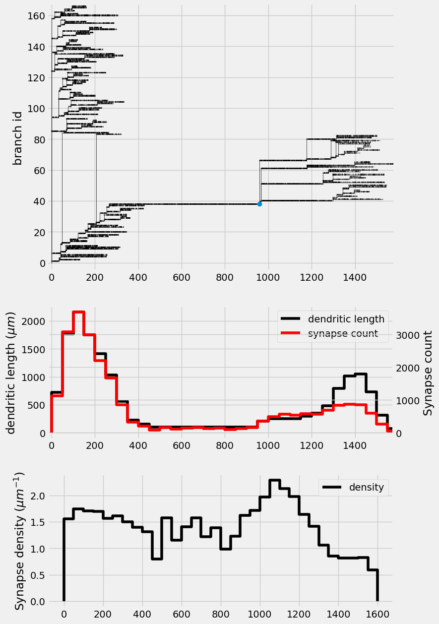
../../_images/tutorials_2._network_models_2.1_Anatomical_embedding_55_0.png

You can also simply plot out the morphology and the synapse locations as a fully featured plot using CellMorphologyVisualizer

[21]:

from visualize.cell_morphology_visualizer import CellMorphologyVisualizer
from matplotlib.pyplot import cm

# only show synapses of this type
synapse_filter = "VPM"
show_synapses = [syntype for syntype in cell.synapses if synapse_filter in syntype]
synapse_colors = cm.Set3(I.np.linspace(0, 1, num=len(show_synapses)))

cmv = CellMorphologyVisualizer(cell)
cmv.population_to_color_dict = dict(zip(show_synapses, synapse_colors))
cmv.background_color="#f0f0f0"
fig, ax = cmv.plot(show_synapses=show_synapses, show_legend=True)

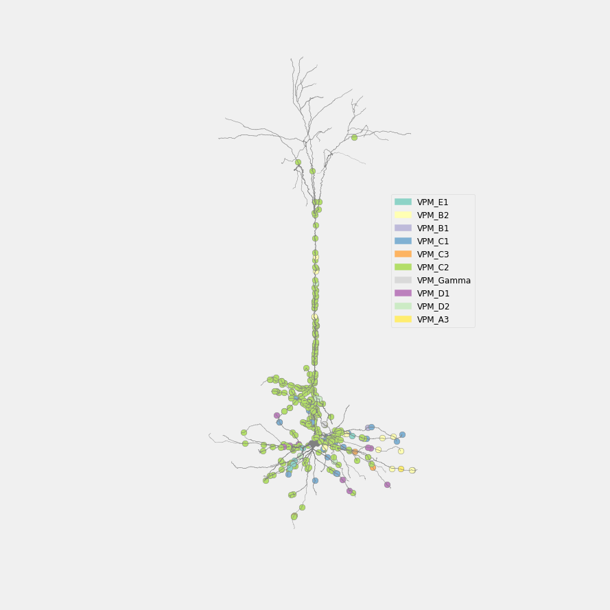
../../_images/tutorials_2._network_models_2.1_Anatomical_embedding_57_0.png

Compatibility with other dense connectome models.¶

While ISF currently only features one network embedding pipeline (Udvary et al., 2022), ISF is not limited to this particular way of generating synapse locations. As long as a .syn and .con file is present (no matter which pipeline created them), any dense connectome model is compatible with ISF. All subsequent workflows in ISF simply rely on these .syn and .con files, but not on the input data that was necessary to generate these. In other words, the barrel cortex model as downloaded in the beginning of this tutorial is simply one example of a network model. Many other dense connectome models may be used. If you have a different way of generating synapse locations, but you still want to use ISF, simply convert the information to .syn and .con. The file formats are purposefully kept as simple as possible.

Recap¶

This tutorial provided a full pipeline on how to generate synapse locations for a given neuron morphology (i.e. an “anatomical network embedding”), and how to parallellize these for multiple morphologies.

In order to assign activity to these synapse realizations, consult the the next tutorial.

Embedding a neuron model in a network model¶

The .syn file¶

The .con file¶

The network parameters¶

Embedding a neuron model into a network model¶

Computing it yourself¶

Copying a pre-computed result instead¶

Parallelizing the generation of anatomical models¶

Client

Cluster

Client

Cluster

Inspecting the output¶

Analyzing and visualizing the network embedding¶

Compatibility with other dense connectome models.¶

Recap¶

The .syn file ¶

The .con file ¶

The network parameters ¶