Network activity
The previous notebook provided us with an anatomical reconstruction of the barrel cortex, defining locations of presynaptic cells, and post-synaptic targets onto our cell. Given this anatomical data, we can now activate the synapses according to experimental data.
To do this, we need the following information
A parameter file specifying characteristics of the synaspses by celltype
A parameterfile specifying the ongoing activity by celltype
Parameterfiles specifying evoked response by stimulus, celltype and cell location
[1]:
from pathlib import Path
tutorial_output_dir = f"{Path.home()}/isf_tutorial_output"  # <-- Change this to your desired output directory
[2]:
import Interface as I
from getting_started import getting_started_dir
%matplotlib inline
[INFO] ISF: Current version: heads/scim+0.ga9c9e61ce.dirty
[INFO] ISF: Current pid: 4188502
[INFO] l5pt: Loaded mechanisms in NEURON namespace.
Warning: no DISPLAY environment variable.
--No graphics will be displayed.
[ATTENTION] ISF: The source folder has uncommited changes!


[INFO] ISF: Loaded modules with __version__ attribute are:
IPython: 8.18.1, Interface: heads/scim+0.ga9c9e61ce.dirty, PIL: 11.3.0, _brotli: 1.1.0, _csv: 1.0, _ctypes: 1.1.0, _curses: b'2.2', _decimal: 1.70, argparse: 1.1, blosc: 1.11.3, bluepyopt: 1.9.126, brotli: 1.1.0, certifi: 2025.08.03, charset_normalizer: 3.4.3, click: 7.1.2, cloudpickle: 3.1.1, colorama: 0.4.6, comm: 0.2.3, csv: 1.0, ctypes: 1.1.0, cycler: 0.12.1, cytoolz: 1.0.1, dash: 2.18.2, dask: 2.30.0, dateutil: 2.9.0.post0, deap: 1.4, debugpy: 1.8.16, decimal: 1.70, decorator: 5.2.1, defusedxml: 0.7.1, distributed: 2.30.0, distutils: 3.9.23, entrypoints: 0.4, exceptiongroup: 1.3.0, executing: 2.2.0, fasteners: 0.17.3, flask: 1.1.4, fsspec: 2025.7.0, future: 1.0.0, greenlet: 3.2.4, idna: 3.10, ipaddress: 1.0, ipykernel: 6.29.5, ipywidgets: 8.1.7, isf_pandas_msgpack: 0.4.0, itsdangerous: 1.1.0, jedi: 0.19.2, jinja2: 2.11.3, joblib: 1.5.1, json: 2.0.9, jupyter_client: 7.3.4, jupyter_core: 5.8.1, kiwisolver: 1.4.7, logging: 0.5.1.2, markupsafe: 2.0.1, matplotlib: 3.3.2, msgpack: 1.1.1, neuron: 7.8.2+, numcodecs: 0.12.1, numexpr: 2.9.0, numpy: 1.19.2, packaging: 25.0, pandas: 1.1.3, parso: 0.8.4, past: 1.0.0, pexpect: 4.9.0, pickleshare: 0.7.5, platform: 1.0.8, platformdirs: 4.3.8, plotly: 5.24.1, prompt_toolkit: 3.0.51, psutil: 7.0.0, ptyprocess: 0.7.0, pure_eval: 0.2.3, pydevd: 3.2.3, pygments: 2.19.2, pyparsing: 3.2.3, pytz: 2025.2, re: 2.2.1, requests: 2.32.5, scipy: 1.5.2, seaborn: 0.12.2, six: 1.17.0, sklearn: 0.23.2, socketserver: 0.4, socks: 1.7.1, sortedcontainers: 2.4.0, stack_data: 0.6.3, statsmodels: 0.12.1, tables: 3.8.0, tblib: 3.1.0, tlz: 1.0.1, toolz: 1.0.0, tqdm: 4.67.1, traitlets: 5.14.3, urllib3: 2.5.0, wcwidth: 0.2.13, werkzeug: 1.0.1, yaml: 6.0.2, zarr: 2.15.0, zlib: 1.0, zmq: 27.0.2, zstandard: 0.23.0
[3]:
I.logger.setLevel("INFO")
Exploring the data
Running simulations with network activity in ISF requires you to know which kind of network activity you would want to simulate.
In the next section, we show how you can build network parameters, containing cell type-specific information on the following:
The network embedding (see the previous tutorial)
Synapse dynamics
Network activity (ongoing and/or evoked)
Before we do that, we will first explore exactly what this data is, and how it should look like for use in ISF
Activity data
Activity data in ISF can be defined in many ways, from distributions (normal, lognormal, uniform), to empirically measured PSTHs.
In this tutorial, we will consider activity data capturing the empirically measured network activity during a specific in vivo condition.
The experimental condition we will consider here is a passive whisker touch of the rat. We have files capturing the activity of all celltypes in all locations across the rat barrel cortex. Let’s see what these files look like:
[4]:
evoked_activity_dir = Path(getting_started_dir) / "example_data" / "functional_constraints" / "evoked_activity"
evoked_activity_files = list(evoked_activity_dir.glob("*.param"))
[str(paramfile.name) for paramfile in evoked_activity_files]
[4]:
['Beta_stim.param',
 'D4_stim.param',
 'E2_stim.param',
 'D3_stim.param',
 'C4_stim.param',
 'B2_stim.param',
 'C2_stim.param',
 'A1_stim.param',
 'A3_stim.param',
 'C1_stim.param',
 'A4_stim.param',
 'E3_stim.param',
 'B4_stim.param',
 'E1_stim.param',
 'C3_stim.param',
 'Delta_stim.param',
 'B3_stim.param',
 'D2_stim.param',
 'Gamma_stim.param',
 'Alpha_stim.param',
 'B1_stim.param',
 'A2_stim.param',
 'D1_stim.param',
 'E4_stim.param']
Let’s check what’s inside these data files
[5]:
I.scp.build_parameters(evoked_activity_files[0]).as_dict()
[5]:
{'L2_B1': {'distribution': 'PSTH',
'intervals': [[3.0, 4.0],
[6.0, 7.0],
[15.0, 16.0],
[37.0, 38.0],
[40.0, 41.0],
[45.0, 46.0],
[46.0, 47.0]],
'probabilities': [0.0013, 0.0013, 0.0013, 0.0013, 0.0013, 0.0013, 0.0013]},
'L2_C1': {'distribution': 'PSTH',
'intervals': [[6.0, 7.0],
[11.0, 12.0],
[19.0, 20.0],
[21.0, 22.0],
[25.0, 26.0]],
'probabilities': [0.0029, 0.0029, 0.0013, 0.0013, 0.0013]},
'L2_Alpha': {'distribution': 'PSTH',
'intervals': [[11.0, 12.0],
[12.0, 13.0],
[13.0, 14.0],
[17.0, 18.0],
[19.0, 20.0],
[33.0, 34.0],
[38.0, 39.0],
[42.0, 43.0],
[45.0, 46.0],
[49.0, 50.0]],
'probabilities': [0.0013,
0.0013,
0.0013,
0.0013,
0.0013,
0.0029,
0.0013,
0.0029,
0.0029,
0.0013]},
'L2_Beta': {'distribution': 'PSTH',
'intervals': [[1.0, 2.0],
[4.0, 5.0],
[5.0, 6.0],
[10.0, 11.0],
[14.0, 15.0],
[16.0, 17.0],
[18.0, 19.0],
[42.0, 43.0],
[43.0, 44.0],
[48.0, 49.0]],
'probabilities': [0.0013,
0.0013,
0.0013,
0.0013,
0.0013,
0.0013,
0.0029,
0.0013,
0.0029,
0.0013]},
'L2_Gamma': {'distribution': 'PSTH',
'intervals': [[4.0, 5.0],
[8.0, 9.0],
[24.0, 25.0],
[27.0, 28.0],
[34.0, 35.0],
[38.0, 39.0],
[39.0, 40.0],
[40.0, 41.0],
[41.0, 42.0],
[42.0, 43.0],
[45.0, 46.0]],
'probabilities': [0.0013,
0.0013,
0.0013,
0.0013,
0.0013,
0.0013,
0.0013,
0.0013,
0.0013,
0.0013,
0.0013]},
'L34_B1': {'distribution': 'PSTH',
'intervals': [[30.0, 31.0],
[32.0, 33.0],
[38.0, 39.0],
[41.0, 42.0],
[46.0, 47.0],
[47.0, 48.0],
[48.0, 49.0]],
'probabilities': [0.0018, 0.0018, 0.0018, 0.0018, 0.0018, 0.0038, 0.0018]},
'L34_C1': {'distribution': 'PSTH',
'intervals': [[2.0, 3.0],
[10.0, 11.0],
[32.0, 33.0],
[40.0, 41.0],
[41.0, 42.0]],
'probabilities': [0.0018, 0.0018, 0.0018, 0.0018, 0.0018]},
'L34_Alpha': {'distribution': 'PSTH',
'intervals': [[2.0, 3.0], [38.0, 39.0]],
'probabilities': [0.0018, 0.0018]},
'L34_Beta': {'distribution': 'PSTH',
'intervals': [[2.0, 3.0],
[8.0, 9.0],
[13.0, 14.0],
[14.0, 15.0],
[16.0, 17.0],
[17.0, 18.0],
[18.0, 19.0],
[19.0, 20.0],
[20.0, 21.0],
[21.0, 22.0],
[22.0, 23.0],
[23.0, 24.0],
[25.0, 26.0],
[28.0, 29.0],
[32.0, 33.0],
[33.0, 34.0],
[35.0, 36.0],
[37.0, 38.0],
[39.0, 40.0],
[41.0, 42.0],
[42.0, 43.0],
[43.0, 44.0],
[45.0, 46.0],
[49.0, 50.0]],
'probabilities': [0.0018,
0.0018,
0.0138,
0.0098,
0.0018,
0.0018,
0.0018,
0.0038,
0.0038,
0.0018,
0.0018,
0.0038,
0.0058,
0.0018,
0.0018,
0.0018,
0.0018,
0.0018,
0.0018,
0.0018,
0.0038,
0.0018,
0.0018,
0.0038]},
'L34_Gamma': {'distribution': 'PSTH',
'intervals': [[39.0, 40.0]],
'probabilities': [0.0018]},
'L4py_B1': {'distribution': 'PSTH',
'intervals': [[5.0, 6.0], [12.0, 13.0], [16.0, 17.0]],
'probabilities': [0.0111, 0.0111, 0.0111]},
'L4py_C1': {'distribution': 'PSTH',
'intervals': [[48.0, 49.0]],
'probabilities': [0.0111]},
'L4py_Alpha': {'distribution': 'PSTH',
'intervals': [[19.0, 20.0], [32.0, 33.0], [43.0, 44.0]],
'probabilities': [0.0111, 0.0111, 0.0111]},
'L4py_Beta': {'distribution': 'PSTH',
'intervals': [[20.0, 21.0], [29.0, 30.0], [40.0, 41.0]],
'probabilities': [0.0111, 0.0111, 0.0111]},
'L4py_Gamma': {'distribution': 'PSTH',
'intervals': [[21.0, 22.0], [23.0, 24.0], [24.0, 25.0], [48.0, 49.0]],
'probabilities': [0.0111, 0.0111, 0.0111, 0.0111]},
'L4sp_B1': {'distribution': 'PSTH', 'intervals': [], 'probabilities': []},
'L4sp_C1': {'distribution': 'PSTH',
'intervals': [[27.0, 28.0]],
'probabilities': [0.0113]},
'L4sp_Alpha': {'distribution': 'PSTH',
'intervals': [[25.0, 26.0], [44.0, 45.0]],
'probabilities': [0.0113, 0.0113]},
'L4sp_Beta': {'distribution': 'PSTH',
'intervals': [[13.0, 14.0],
[14.0, 15.0],
[15.0, 16.0],
[30.0, 31.0],
[35.0, 36.0],
[36.0, 37.0],
[41.0, 42.0]],
'probabilities': [0.057, 0.0227, 0.0227, 0.0113, 0.0113, 0.0113, 0.0113]},
'L4sp_Gamma': {'distribution': 'PSTH', 'intervals': [], 'probabilities': []},
'L4ss_B1': {'distribution': 'PSTH',
'intervals': [[0.0, 1.0],
[15.0, 16.0],
[16.0, 17.0],
[17.0, 18.0],
[18.0, 19.0],
[19.0, 20.0],
[20.0, 21.0],
[21.0, 22.0],
[22.0, 23.0],
[23.0, 24.0],
[25.0, 26.0],
[28.0, 29.0],
[30.0, 31.0],
[31.0, 32.0],
[32.0, 33.0],
[33.0, 34.0],
[37.0, 38.0],
[39.0, 40.0],
[40.0, 41.0],
[41.0, 42.0],
[44.0, 45.0],
[45.0, 46.0]],
'probabilities': [0.0029,
0.0059,
0.015,
0.0059,
0.0059,
0.012,
0.0059,
0.0029,
0.015,
0.0029,
0.0029,
0.0059,
0.0029,
0.0059,
0.0089,
0.0029,
0.0029,
0.0029,
0.0029,
0.0029,
0.0029,
0.0029]},
'L4ss_C1': {'distribution': 'PSTH',
'intervals': [[34.0, 35.0],
[35.0, 36.0],
[37.0, 38.0],
[38.0, 39.0],
[41.0, 42.0],
[45.0, 46.0],
[46.0, 47.0]],
'probabilities': [0.0029, 0.0029, 0.0059, 0.0029, 0.0029, 0.0029, 0.0029]},
'L4ss_Alpha': {'distribution': 'PSTH', 'intervals': [], 'probabilities': []},
'L4ss_Beta': {'distribution': 'PSTH',
'intervals': [[9.0, 10.0],
[11.0, 12.0],
[12.0, 13.0],
[17.0, 18.0],
[20.0, 21.0],
[24.0, 25.0],
[27.0, 28.0],
[28.0, 29.0],
[30.0, 31.0],
[32.0, 33.0],
[33.0, 34.0],
[34.0, 35.0],
[35.0, 36.0],
[36.0, 37.0],
[37.0, 38.0],
[38.0, 39.0],
[39.0, 40.0],
[41.0, 42.0],
[42.0, 43.0],
[44.0, 45.0],
[45.0, 46.0]],
'probabilities': [0.0029,
0.0089,
0.015,
0.0029,
0.0029,
0.0059,
0.0029,
0.0029,
0.0059,
0.0059,
0.0059,
0.0029,
0.0089,
0.0029,
0.0059,
0.0059,
0.0059,
0.0029,
0.0089,
0.0089,
0.0029]},
'L4ss_Gamma': {'distribution': 'PSTH',
'intervals': [[1.0, 2.0],
[24.0, 25.0],
[31.0, 32.0],
[34.0, 35.0],
[35.0, 36.0],
[36.0, 37.0],
[41.0, 42.0],
[44.0, 45.0]],
'probabilities': [0.0029,
0.0029,
0.0029,
0.0059,
0.0029,
0.0029,
0.0029,
0.0029]},
'L5st_B1': {'distribution': 'PSTH',
'intervals': [[2.0, 3.0],
[10.0, 11.0],
[12.0, 13.0],
[14.0, 15.0],
[25.0, 26.0],
[27.0, 28.0],
[28.0, 29.0],
[34.0, 35.0],
[36.0, 37.0],
[37.0, 38.0],
[38.0, 39.0],
[39.0, 40.0],
[41.0, 42.0],
[46.0, 47.0],
[48.0, 49.0]],
'probabilities': [0.0007,
0.0007,
0.0007,
0.0007,
0.0007,
0.0007,
0.0019,
0.0031,
0.0031,
0.0031,
0.0007,
0.0007,
0.0055,
0.0019,
0.0007]},
'L5st_C1': {'distribution': 'PSTH',
'intervals': [[3.0, 4.0],
[5.0, 6.0],
[6.0, 7.0],
[9.0, 10.0],
[10.0, 11.0],
[12.0, 13.0],
[13.0, 14.0],
[15.0, 16.0],
[16.0, 17.0],
[17.0, 18.0],
[24.0, 25.0],
[25.0, 26.0],
[29.0, 30.0],
[30.0, 31.0],
[37.0, 38.0],
[38.0, 39.0],
[39.0, 40.0],
[42.0, 43.0],
[43.0, 44.0],
[45.0, 46.0],
[46.0, 47.0],
[49.0, 50.0]],
'probabilities': [0.0007,
0.0007,
0.0007,
0.0007,
0.0007,
0.0019,
0.0019,
0.0007,
0.0019,
0.0007,
0.0007,
0.0007,
0.0019,
0.0007,
0.0019,
0.0007,
0.0007,
0.0007,
0.0007,
0.0019,
0.0031,
0.0007]},
'L5st_Alpha': {'distribution': 'PSTH',
'intervals': [[0.0, 1.0],
[3.0, 4.0],
[6.0, 7.0],
[12.0, 13.0],
[13.0, 14.0],
[14.0, 15.0],
[15.0, 16.0],
[16.0, 17.0],
[17.0, 18.0],
[19.0, 20.0],
[23.0, 24.0],
[25.0, 26.0],
[29.0, 30.0],
[33.0, 34.0],
[34.0, 35.0],
[35.0, 36.0],
[37.0, 38.0],
[38.0, 39.0],
[41.0, 42.0],
[44.0, 45.0],
[45.0, 46.0],
[47.0, 48.0],
[48.0, 49.0]],
'probabilities': [0.0007,
0.0007,
0.0007,
0.0007,
0.0007,
0.0019,
0.0007,
0.0031,
0.0007,
0.0007,
0.0007,
0.0007,
0.0007,
0.0007,
0.0019,
0.0007,
0.0007,
0.0007,
0.0007,
0.0007,
0.0007,
0.0019,
0.0007]},
'L5st_Beta': {'distribution': 'PSTH',
'intervals': [[10.0, 11.0],
[13.0, 14.0],
[14.0, 15.0],
[15.0, 16.0],
[20.0, 21.0],
[22.0, 23.0],
[26.0, 27.0],
[27.0, 28.0],
[29.0, 30.0],
[32.0, 33.0],
[34.0, 35.0],
[35.0, 36.0],
[37.0, 38.0],
[41.0, 42.0],
[42.0, 43.0],
[44.0, 45.0],
[45.0, 46.0],
[46.0, 47.0],
[48.0, 49.0],
[49.0, 50.0]],
'probabilities': [0.0031,
0.0019,
0.0007,
0.0019,
0.0007,
0.0031,
0.0019,
0.0007,
0.0007,
0.0007,
0.0007,
0.0007,
0.0007,
0.0007,
0.0019,
0.0007,
0.0007,
0.0007,
0.0043,
0.0055]},
'L5st_Gamma': {'distribution': 'PSTH',
'intervals': [[1.0, 2.0],
[5.0, 6.0],
[8.0, 9.0],
[9.0, 10.0],
[10.0, 11.0],
[12.0, 13.0],
[16.0, 17.0],
[17.0, 18.0],
[19.0, 20.0],
[21.0, 22.0],
[22.0, 23.0],
[23.0, 24.0],
[27.0, 28.0],
[28.0, 29.0],
[30.0, 31.0],
[32.0, 33.0],
[33.0, 34.0],
[37.0, 38.0],
[38.0, 39.0],
[39.0, 40.0],
[42.0, 43.0],
[43.0, 44.0],
[44.0, 45.0],
[47.0, 48.0],
[48.0, 49.0]],
'probabilities': [0.0007,
0.0007,
0.0007,
0.0007,
0.0007,
0.0007,
0.0019,
0.0019,
0.0007,
0.0007,
0.0007,
0.0007,
0.0007,
0.0007,
0.0007,
0.0007,
0.0007,
0.0007,
0.0007,
0.0019,
0.0007,
0.0007,
0.0019,
0.0019,
0.0007]},
'L5tt_B1': {'distribution': 'PSTH',
'intervals': [[2.0, 3.0],
[3.0, 4.0],
[6.0, 7.0],
[7.0, 8.0],
[8.0, 9.0],
[9.0, 10.0],
[10.0, 11.0],
[13.0, 14.0],
[14.0, 15.0],
[15.0, 16.0],
[16.0, 17.0],
[17.0, 18.0],
[18.0, 19.0],
[19.0, 20.0],
[20.0, 21.0],
[21.0, 22.0],
[22.0, 23.0],
[23.0, 24.0],
[24.0, 25.0],
[26.0, 27.0],
[29.0, 30.0],
[30.0, 31.0],
[31.0, 32.0],
[32.0, 33.0],
[33.0, 34.0],
[34.0, 35.0],
[35.0, 36.0],
[37.0, 38.0],
[38.0, 39.0],
[39.0, 40.0],
[40.0, 41.0],
[41.0, 42.0],
[42.0, 43.0],
[43.0, 44.0],
[45.0, 46.0],
[46.0, 47.0],
[47.0, 48.0],
[48.0, 49.0],
[49.0, 50.0]],
'probabilities': [0.0009,
0.0009,
0.0009,
0.0009,
0.0035,
0.0009,
0.0035,
0.0162,
0.0162,
0.006,
0.006,
0.006,
0.0111,
0.0187,
0.0136,
0.0009,
0.006,
0.0035,
0.0086,
0.006,
0.0086,
0.0035,
0.0009,
0.0162,
0.0009,
0.006,
0.0035,
0.0035,
0.006,
0.0035,
0.006,
0.0035,
0.006,
0.0009,
0.0035,
0.0009,
0.0009,
0.0035,
0.0035]},
'L5tt_C1': {'distribution': 'PSTH',
'intervals': [[3.0, 4.0],
[4.0, 5.0],
[6.0, 7.0],
[12.0, 13.0],
[14.0, 15.0],
[17.0, 18.0],
[18.0, 19.0],
[19.0, 20.0],
[20.0, 21.0],
[21.0, 22.0],
[22.0, 23.0],
[23.0, 24.0],
[24.0, 25.0],
[26.0, 27.0],
[27.0, 28.0],
[28.0, 29.0],
[29.0, 30.0],
[31.0, 32.0],
[35.0, 36.0],
[36.0, 37.0],
[37.0, 38.0],
[39.0, 40.0],
[41.0, 42.0],
[43.0, 44.0],
[44.0, 45.0],
[45.0, 46.0],
[46.0, 47.0],
[48.0, 49.0],
[49.0, 50.0]],
'probabilities': [0.0009,
0.0009,
0.0009,
0.0009,
0.0009,
0.006,
0.0111,
0.0035,
0.006,
0.0086,
0.0009,
0.0035,
0.006,
0.0035,
0.0009,
0.006,
0.0035,
0.006,
0.0111,
0.0035,
0.0086,
0.0009,
0.0035,
0.0009,
0.0035,
0.0086,
0.006,
0.0035,
0.0035]},
'L5tt_Alpha': {'distribution': 'PSTH',
'intervals': [[0.0, 1.0],
[4.0, 5.0],
[8.0, 9.0],
[12.0, 13.0],
[13.0, 14.0],
[14.0, 15.0],
[15.0, 16.0],
[16.0, 17.0],
[17.0, 18.0],
[19.0, 20.0],
[20.0, 21.0],
[21.0, 22.0],
[22.0, 23.0],
[23.0, 24.0],
[24.0, 25.0],
[25.0, 26.0],
[26.0, 27.0],
[28.0, 29.0],
[30.0, 31.0],
[31.0, 32.0],
[33.0, 34.0],
[34.0, 35.0],
[35.0, 36.0],
[36.0, 37.0],
[37.0, 38.0],
[38.0, 39.0],
[39.0, 40.0],
[40.0, 41.0],
[41.0, 42.0],
[42.0, 43.0],
[43.0, 44.0],
[44.0, 45.0],
[46.0, 47.0],
[47.0, 48.0],
[48.0, 49.0],
[49.0, 50.0]],
'probabilities': [0.0009,
0.0009,
0.0009,
0.0086,
0.0162,
0.0162,
0.0035,
0.0086,
0.0035,
0.0035,
0.0009,
0.0009,
0.0035,
0.006,
0.0009,
0.0009,
0.0035,
0.006,
0.0035,
0.0086,
0.0009,
0.006,
0.0035,
0.0035,
0.0086,
0.0035,
0.0009,
0.006,
0.0009,
0.0035,
0.0035,
0.0111,
0.0009,
0.0035,
0.0035,
0.0035]},
'L5tt_Beta': {'distribution': 'PSTH',
'intervals': [[5.0, 6.0],
[9.0, 10.0],
[11.0, 12.0],
[12.0, 13.0],
[13.0, 14.0],
[14.0, 15.0],
[15.0, 16.0],
[16.0, 17.0],
[18.0, 19.0],
[19.0, 20.0],
[20.0, 21.0],
[21.0, 22.0],
[22.0, 23.0],
[23.0, 24.0],
[24.0, 25.0],
[25.0, 26.0],
[26.0, 27.0],
[27.0, 28.0],
[28.0, 29.0],
[29.0, 30.0],
[31.0, 32.0],
[32.0, 33.0],
[33.0, 34.0],
[34.0, 35.0],
[35.0, 36.0],
[37.0, 38.0],
[38.0, 39.0],
[40.0, 41.0],
[41.0, 42.0],
[43.0, 44.0],
[44.0, 45.0],
[45.0, 46.0],
[46.0, 47.0],
[47.0, 48.0],
[48.0, 49.0],
[49.0, 50.0]],
'probabilities': [0.0009,
0.0009,
0.0035,
0.0111,
0.034,
0.0263,
0.0162,
0.006,
0.0035,
0.0111,
0.0035,
0.0009,
0.0009,
0.0009,
0.0086,
0.0035,
0.0009,
0.006,
0.0035,
0.0035,
0.0009,
0.0086,
0.0009,
0.0009,
0.0009,
0.0009,
0.006,
0.006,
0.0035,
0.0035,
0.0009,
0.006,
0.0035,
0.0009,
0.0035,
0.0009]},
'L5tt_Gamma': {'distribution': 'PSTH',
'intervals': [[0.0, 1.0],
[2.0, 3.0],
[5.0, 6.0],
[6.0, 7.0],
[7.0, 8.0],
[9.0, 10.0],
[13.0, 14.0],
[14.0, 15.0],
[15.0, 16.0],
[16.0, 17.0],
[17.0, 18.0],
[18.0, 19.0],
[19.0, 20.0],
[20.0, 21.0],
[21.0, 22.0],
[22.0, 23.0],
[23.0, 24.0],
[26.0, 27.0],
[28.0, 29.0],
[29.0, 30.0],
[30.0, 31.0],
[32.0, 33.0],
[33.0, 34.0],
[34.0, 35.0],
[35.0, 36.0],
[36.0, 37.0],
[37.0, 38.0],
[38.0, 39.0],
[42.0, 43.0],
[44.0, 45.0],
[45.0, 46.0],
[46.0, 47.0],
[47.0, 48.0],
[48.0, 49.0],
[49.0, 50.0]],
'probabilities': [0.0035,
0.0035,
0.0009,
0.0035,
0.0035,
0.0009,
0.0009,
0.0035,
0.0009,
0.0035,
0.0035,
0.0009,
0.0136,
0.0009,
0.006,
0.0136,
0.0009,
0.0035,
0.0009,
0.0009,
0.0009,
0.0035,
0.0009,
0.0035,
0.006,
0.0009,
0.0035,
0.0035,
0.0009,
0.0009,
0.006,
0.0035,
0.0009,
0.0035,
0.0009]},
'L6cc_B1': {'distribution': 'PSTH',
'intervals': [[7.0, 8.0],
[8.0, 9.0],
[9.0, 10.0],
[10.0, 11.0],
[11.0, 12.0],
[12.0, 13.0],
[13.0, 14.0],
[16.0, 17.0],
[18.0, 19.0],
[20.0, 21.0],
[27.0, 28.0],
[31.0, 32.0],
[33.0, 34.0],
[34.0, 35.0],
[36.0, 37.0],
[38.0, 39.0],
[40.0, 41.0],
[42.0, 43.0],
[48.0, 49.0]],
'probabilities': [0.0034,
0.0034,
0.0148,
0.0681,
0.0377,
0.011,
0.0034,
0.0072,
0.0072,
0.0034,
0.0034,
0.0034,
0.0072,
0.0072,
0.0034,
0.0034,
0.0034,
0.0034,
0.0034]},
'L6cc_C1': {'distribution': 'PSTH',
'intervals': [[10.0, 11.0],
[11.0, 12.0],
[20.0, 21.0],
[22.0, 23.0],
[32.0, 33.0],
[33.0, 34.0],
[34.0, 35.0],
[36.0, 37.0],
[37.0, 38.0],
[41.0, 42.0],
[43.0, 44.0],
[45.0, 46.0]],
'probabilities': [0.0034,
0.0034,
0.0072,
0.0034,
0.0034,
0.0034,
0.0034,
0.0034,
0.0034,
0.0034,
0.0034,
0.0034]},
'L6cc_Alpha': {'distribution': 'PSTH',
'intervals': [[9.0, 10.0],
[10.0, 11.0],
[30.0, 31.0],
[37.0, 38.0],
[41.0, 42.0],
[42.0, 43.0],
[43.0, 44.0],
[45.0, 46.0],
[48.0, 49.0]],
'probabilities': [0.0034,
0.0034,
0.0034,
0.0072,
0.0034,
0.0034,
0.0034,
0.0034,
0.0072]},
'L6cc_Beta': {'distribution': 'PSTH',
'intervals': [[3.0, 4.0],
[6.0, 7.0],
[9.0, 10.0],
[10.0, 11.0],
[11.0, 12.0],
[12.0, 13.0],
[13.0, 14.0],
[14.0, 15.0],
[15.0, 16.0],
[18.0, 19.0],
[19.0, 20.0],
[33.0, 34.0],
[34.0, 35.0],
[35.0, 36.0],
[36.0, 37.0],
[41.0, 42.0],
[42.0, 43.0],
[43.0, 44.0]],
'probabilities': [0.0034,
0.0034,
0.0186,
0.0757,
0.0491,
0.0186,
0.0034,
0.0034,
0.0072,
0.0034,
0.0034,
0.0072,
0.0034,
0.0072,
0.0034,
0.0034,
0.0072,
0.0034]},
'L6cc_Gamma': {'distribution': 'PSTH',
'intervals': [[10.0, 11.0],
[17.0, 18.0],
[20.0, 21.0],
[25.0, 26.0],
[34.0, 35.0],
[36.0, 37.0],
[37.0, 38.0],
[41.0, 42.0]],
'probabilities': [0.0034,
0.0034,
0.0072,
0.0034,
0.0034,
0.0034,
0.0034,
0.0072]},
'L6ccinv_B1': {'distribution': 'PSTH', 'intervals': [], 'probabilities': []},
'L6ccinv_C1': {'distribution': 'PSTH',
'intervals': [[41.0, 42.0], [45.0, 46.0]],
'probabilities': [0.0227, 0.0227]},
'L6ccinv_Alpha': {'distribution': 'PSTH',
'intervals': [],
'probabilities': []},
'L6ccinv_Beta': {'distribution': 'PSTH',
'intervals': [[35.0, 36.0]],
'probabilities': [0.0227]},
'L6ccinv_Gamma': {'distribution': 'PSTH',
'intervals': [],
'probabilities': []},
'L6ct_B1': {'distribution': 'PSTH',
'intervals': [[21.0, 22.0],
[32.0, 33.0],
[34.0, 35.0],
[39.0, 40.0],
[42.0, 43.0]],
'probabilities': [0.0045, 0.0045, 0.0045, 0.0045, 0.0045]},
'L6ct_C1': {'distribution': 'PSTH',
'intervals': [[40.0, 41.0]],
'probabilities': [0.0045]},
'L6ct_Alpha': {'distribution': 'PSTH',
'intervals': [[38.0, 39.0]],
'probabilities': [0.0045]},
'L6ct_Beta': {'distribution': 'PSTH',
'intervals': [[17.0, 18.0],
[20.0, 21.0],
[23.0, 24.0],
[25.0, 26.0],
[26.0, 27.0],
[27.0, 28.0],
[29.0, 30.0],
[32.0, 33.0],
[34.0, 35.0],
[35.0, 36.0],
[40.0, 41.0]],
'probabilities': [0.0045,
0.0091,
0.0045,
0.0045,
0.0045,
0.0045,
0.0045,
0.0045,
0.0045,
0.0045,
0.0045]},
'L6ct_Gamma': {'distribution': 'PSTH',
'intervals': [[5.0, 6.0]],
'probabilities': [0.0045]},
'VPM_B1': {'distribution': 'PSTH',
'intervals': [[13.0, 17.0]],
'probabilities': [0.049]},
'VPM_C1': {'distribution': 'PSTH',
'intervals': [[13.0, 17.0]],
'probabilities': [0.025]},
'VPM_Alpha': {'distribution': 'PSTH',
'intervals': [[13.0, 17.0]],
'probabilities': [0.012]},
'VPM_Beta': {'distribution': 'PSTH',
'intervals': [[8.0, 10.0], [10.0, 14.9]],
'probabilities': [0.2664, 0.2784]},
'VPM_Gamma': {'distribution': 'PSTH',
'intervals': [[13.0, 17.0]],
'probabilities': [0.033]},
'L1_B1': {'distribution': 'PSTH', 'intervals': [], 'probabilities': []},
'L1_C1': {'distribution': 'PSTH', 'intervals': [], 'probabilities': []},
'L1_Alpha': {'distribution': 'PSTH', 'intervals': [], 'probabilities': []},
'L1_Beta': {'distribution': 'PSTH',
'intervals': [[10.0, 20.0]],
'probabilities': [0.072]},
'L1_Gamma': {'distribution': 'PSTH', 'intervals': [], 'probabilities': []},
'L23Trans_B1': {'distribution': 'PSTH',
'intervals': [[0.0, 1.0],
[2.0, 3.0],
[3.0, 4.0],
[6.0, 7.0],
[7.0, 8.0],
[8.0, 9.0],
[9.0, 10.0],
[10.0, 11.0],
[11.0, 12.0],
[12.0, 13.0],
[13.0, 14.0],
[14.0, 15.0],
[15.0, 16.0],
[16.0, 17.0],
[17.0, 18.0],
[18.0, 19.0],
[19.0, 20.0],
[20.0, 21.0],
[21.0, 22.0],
[22.0, 23.0],
[23.0, 24.0],
[24.0, 25.0],
[25.0, 26.0],
[26.0, 27.0],
[27.0, 28.0],
[28.0, 29.0],
[29.0, 30.0],
[30.0, 31.0],
[31.0, 32.0],
[32.0, 33.0],
[33.0, 34.0],
[34.0, 35.0],
[35.0, 36.0],
[36.0, 37.0],
[37.0, 38.0],
[38.0, 39.0],
[39.0, 40.0],
[40.0, 41.0],
[41.0, 42.0],
[42.0, 43.0],
[43.0, 44.0],
[44.0, 45.0],
[45.0, 46.0],
[46.0, 47.0],
[47.0, 48.0],
[48.0, 49.0],
[49.0, 50.0]],
'probabilities': [0.0035,
0.0012,
0.0012,
0.0012,
0.0042,
0.0043,
0.0183,
0.0841,
0.0465,
0.0135,
0.02,
0.02,
0.0152,
0.0186,
0.0074,
0.0137,
0.0231,
0.0168,
0.0035,
0.0186,
0.0043,
0.0106,
0.0035,
0.0074,
0.0042,
0.0073,
0.0106,
0.0043,
0.0073,
0.02,
0.0089,
0.0089,
0.0043,
0.0042,
0.0043,
0.0074,
0.0043,
0.0074,
0.0043,
0.0074,
0.0012,
0.0035,
0.0043,
0.0023,
0.0047,
0.0043,
0.0043]},
'L23Trans_C1': {'distribution': 'PSTH',
'intervals': [[2.0, 3.0],
[3.0, 4.0],
[4.0, 5.0],
[6.0, 7.0],
[10.0, 11.0],
[11.0, 12.0],
[12.0, 13.0],
[13.0, 14.0],
[14.0, 15.0],
[15.0, 16.0],
[16.0, 17.0],
[17.0, 18.0],
[18.0, 19.0],
[19.0, 20.0],
[20.0, 21.0],
[21.0, 22.0],
[22.0, 23.0],
[23.0, 24.0],
[24.0, 25.0],
[26.0, 27.0],
[27.0, 28.0],
[28.0, 29.0],
[29.0, 30.0],
[31.0, 32.0],
[32.0, 33.0],
[33.0, 34.0],
[34.0, 35.0],
[35.0, 36.0],
[36.0, 37.0],
[37.0, 38.0],
[38.0, 39.0],
[39.0, 40.0],
[40.0, 41.0],
[41.0, 42.0],
[43.0, 44.0],
[44.0, 45.0],
[45.0, 46.0],
[46.0, 47.0],
[48.0, 49.0],
[49.0, 50.0]],
'probabilities': [0.0049,
0.0026,
0.0026,
0.0026,
0.009,
0.009,
0.0026,
0.0168,
0.0168,
0.0168,
0.0168,
0.0161,
0.0296,
0.0092,
0.0191,
0.0227,
0.009,
0.0092,
0.0161,
0.0092,
0.03,
0.0161,
0.0092,
0.0161,
0.009,
0.009,
0.009,
0.0296,
0.0092,
0.0227,
0.0075,
0.0026,
0.0049,
0.0092,
0.009,
0.0092,
0.0227,
0.0161,
0.0092,
0.0092]},
'L23Trans_Alpha': {'distribution': 'PSTH',
'intervals': [[0.0, 1.0],
[2.0, 3.0],
[4.0, 5.0],
[8.0, 9.0],
[9.0, 10.0],
[10.0, 11.0],
[12.0, 13.0],
[13.0, 14.0],
[14.0, 15.0],
[15.0, 16.0],
[16.0, 17.0],
[17.0, 18.0],
[19.0, 20.0],
[20.0, 21.0],
[21.0, 22.0],
[22.0, 23.0],
[23.0, 24.0],
[24.0, 25.0],
[25.0, 26.0],
[26.0, 27.0],
[28.0, 29.0],
[30.0, 31.0],
[31.0, 32.0],
[33.0, 34.0],
[34.0, 35.0],
[35.0, 36.0],
[36.0, 37.0],
[37.0, 38.0],
[38.0, 39.0],
[39.0, 40.0],
[40.0, 41.0],
[41.0, 42.0],
[42.0, 43.0],
[43.0, 44.0],
[44.0, 45.0],
[45.0, 46.0],
[46.0, 47.0],
[47.0, 48.0],
[48.0, 49.0],
[49.0, 50.0]],
'probabilities': [0.0025,
0.0048,
0.0025,
0.0025,
0.0089,
0.0089,
0.0225,
0.0427,
0.0427,
0.0092,
0.0225,
0.0092,
0.0092,
0.0025,
0.0025,
0.0092,
0.0159,
0.0025,
0.0298,
0.0092,
0.0159,
0.0092,
0.0225,
0.0025,
0.0159,
0.0092,
0.0092,
0.0225,
0.0092,
0.0025,
0.0159,
0.0089,
0.0092,
0.0092,
0.0298,
0.0089,
0.0025,
0.0092,
0.0189,
0.0092]},
'L23Trans_Beta': {'distribution': 'PSTH',
'intervals': [[1.0, 2.0],
[2.0, 3.0],
[4.0, 5.0],
[5.0, 6.0],
[8.0, 9.0],
[9.0, 10.0],
[10.0, 11.0],
[11.0, 12.0],
[12.0, 13.0],
[13.0, 14.0],
[14.0, 15.0],
[15.0, 16.0],
[16.0, 17.0],
[17.0, 18.0],
[18.0, 19.0],
[19.0, 20.0],
[20.0, 21.0],
[21.0, 22.0],
[22.0, 23.0],
[23.0, 24.0],
[24.0, 25.0],
[25.0, 26.0],
[26.0, 27.0],
[27.0, 28.0],
[28.0, 29.0],
[29.0, 30.0],
[30.0, 31.0],
[31.0, 32.0],
[32.0, 33.0],
[33.0, 34.0],
[34.0, 35.0],
[35.0, 36.0],
[36.0, 37.0],
[37.0, 38.0],
[38.0, 39.0],
[39.0, 40.0],
[40.0, 41.0],
[41.0, 42.0],
[42.0, 43.0],
[43.0, 44.0],
[44.0, 45.0],
[45.0, 46.0],
[46.0, 47.0],
[47.0, 48.0],
[48.0, 49.0]],
'probabilities': [0.0023,
0.0043,
0.0012,
0.0043,
0.3373,
0.0959,
0.0705,
0.0705,
0.0722,
0.0705,
0.0288,
0.0076,
0.0036,
0.0044,
0.0141,
0.0049,
0.0023,
0.0023,
0.0049,
0.0108,
0.0073,
0.0012,
0.0076,
0.0044,
0.0044,
0.0143,
0.0012,
0.0108,
0.0091,
0.0043,
0.0143,
0.0143,
0.0075,
0.0076,
0.0075,
0.0076,
0.0143,
0.0113,
0.0044,
0.0113,
0.0076,
0.0044,
0.0012,
0.0044,
0.0049]},
'L23Trans_Gamma': {'distribution': 'PSTH',
'intervals': [[0.0, 1.0],
[1.0, 2.0],
[2.0, 3.0],
[5.0, 6.0],
[6.0, 7.0],
[7.0, 8.0],
[9.0, 10.0],
[10.0, 11.0],
[13.0, 14.0],
[14.0, 15.0],
[15.0, 16.0],
[16.0, 17.0],
[17.0, 18.0],
[18.0, 19.0],
[19.0, 20.0],
[20.0, 21.0],
[21.0, 22.0],
[22.0, 23.0],
[23.0, 24.0],
[24.0, 25.0],
[25.0, 26.0],
[26.0, 27.0],
[28.0, 29.0],
[29.0, 30.0],
[30.0, 31.0],
[31.0, 32.0],
[32.0, 33.0],
[33.0, 34.0],
[34.0, 35.0],
[35.0, 36.0],
[36.0, 37.0],
[37.0, 38.0],
[38.0, 39.0],
[39.0, 40.0],
[41.0, 42.0],
[42.0, 43.0],
[44.0, 45.0],
[45.0, 46.0],
[46.0, 47.0],
[47.0, 48.0],
[48.0, 49.0],
[49.0, 50.0]],
'probabilities': [0.0102,
0.0083,
0.0102,
0.0028,
0.0102,
0.0102,
0.0028,
0.0099,
0.0243,
0.0243,
0.0243,
0.0243,
0.0102,
0.0028,
0.0399,
0.021,
0.0177,
0.0399,
0.0028,
0.0083,
0.0099,
0.0102,
0.0028,
0.0028,
0.0028,
0.0083,
0.0102,
0.0028,
0.0173,
0.0177,
0.0099,
0.0102,
0.0102,
0.0053,
0.021,
0.0028,
0.0083,
0.0177,
0.0102,
0.0028,
0.0102,
0.0028]},
'L45Peak_B1': {'distribution': 'PSTH',
'intervals': [[0.0, 1.0],
[2.0, 3.0],
[3.0, 4.0],
[6.0, 7.0],
[7.0, 8.0],
[8.0, 9.0],
[9.0, 10.0],
[10.0, 11.0],
[11.0, 12.0],
[12.0, 13.0],
[13.0, 14.0],
[14.0, 15.0],
[15.0, 16.0],
[16.0, 17.0],
[17.0, 18.0],
[18.0, 19.0],
[19.0, 20.0],
[20.0, 21.0],
[21.0, 22.0],
[22.0, 23.0],
[23.0, 24.0],
[24.0, 25.0],
[25.0, 26.0],
[26.0, 27.0],
[27.0, 28.0],
[28.0, 29.0],
[29.0, 30.0],
[30.0, 31.0],
[31.0, 32.0],
[32.0, 33.0],
[33.0, 34.0],
[34.0, 35.0],
[35.0, 36.0],
[36.0, 37.0],
[37.0, 38.0],
[38.0, 39.0],
[39.0, 40.0],
[40.0, 41.0],
[41.0, 42.0],
[42.0, 43.0],
[43.0, 44.0],
[44.0, 45.0],
[45.0, 46.0],
[46.0, 47.0],
[47.0, 48.0],
[48.0, 49.0],
[49.0, 50.0]],
'probabilities': [0.0035,
0.0012,
0.0012,
0.0012,
0.0042,
0.0043,
0.0183,
0.0841,
0.0465,
0.0135,
0.02,
0.02,
0.0152,
0.0186,
0.0074,
0.0137,
0.0231,
0.0168,
0.0035,
0.0186,
0.0043,
0.0106,
0.0035,
0.0074,
0.0042,
0.0073,
0.0106,
0.0043,
0.0073,
0.02,
0.0089,
0.0089,
0.0043,
0.0042,
0.0043,
0.0074,
0.0043,
0.0074,
0.0043,
0.0074,
0.0012,
0.0035,
0.0043,
0.0023,
0.0047,
0.0043,
0.0043]},
'L45Peak_C1': {'distribution': 'PSTH',
'intervals': [[2.0, 3.0],
[3.0, 4.0],
[4.0, 5.0],
[6.0, 7.0],
[10.0, 11.0],
[11.0, 12.0],
[12.0, 13.0],
[13.0, 14.0],
[14.0, 15.0],
[15.0, 16.0],
[16.0, 17.0],
[17.0, 18.0],
[18.0, 19.0],
[19.0, 20.0],
[20.0, 21.0],
[21.0, 22.0],
[22.0, 23.0],
[23.0, 24.0],
[24.0, 25.0],
[26.0, 27.0],
[27.0, 28.0],
[28.0, 29.0],
[29.0, 30.0],
[31.0, 32.0],
[32.0, 33.0],
[33.0, 34.0],
[34.0, 35.0],
[35.0, 36.0],
[36.0, 37.0],
[37.0, 38.0],
[38.0, 39.0],
[39.0, 40.0],
[40.0, 41.0],
[41.0, 42.0],
[43.0, 44.0],
[44.0, 45.0],
[45.0, 46.0],
[46.0, 47.0],
[48.0, 49.0],
[49.0, 50.0]],
'probabilities': [0.0049,
0.0026,
0.0026,
0.0026,
0.009,
0.009,
0.0026,
0.0168,
0.0168,
0.0168,
0.0168,
0.0161,
0.0296,
0.0092,
0.0191,
0.0227,
0.009,
0.0092,
0.0161,
0.0092,
0.03,
0.0161,
0.0092,
0.0161,
0.009,
0.009,
0.009,
0.0296,
0.0092,
0.0227,
0.0075,
0.0026,
0.0049,
0.0092,
0.009,
0.0092,
0.0227,
0.0161,
0.0092,
0.0092]},
'L45Peak_Alpha': {'distribution': 'PSTH',
'intervals': [[0.0, 1.0],
[2.0, 3.0],
[4.0, 5.0],
[8.0, 9.0],
[9.0, 10.0],
[10.0, 11.0],
[12.0, 13.0],
[13.0, 14.0],
[14.0, 15.0],
[15.0, 16.0],
[16.0, 17.0],
[17.0, 18.0],
[19.0, 20.0],
[20.0, 21.0],
[21.0, 22.0],
[22.0, 23.0],
[23.0, 24.0],
[24.0, 25.0],
[25.0, 26.0],
[26.0, 27.0],
[28.0, 29.0],
[30.0, 31.0],
[31.0, 32.0],
[33.0, 34.0],
[34.0, 35.0],
[35.0, 36.0],
[36.0, 37.0],
[37.0, 38.0],
[38.0, 39.0],
[39.0, 40.0],
[40.0, 41.0],
[41.0, 42.0],
[42.0, 43.0],
[43.0, 44.0],
[44.0, 45.0],
[45.0, 46.0],
[46.0, 47.0],
[47.0, 48.0],
[48.0, 49.0],
[49.0, 50.0]],
'probabilities': [0.0025,
0.0048,
0.0025,
0.0025,
0.0089,
0.0089,
0.0225,
0.0427,
0.0427,
0.0092,
0.0225,
0.0092,
0.0092,
0.0025,
0.0025,
0.0092,
0.0159,
0.0025,
0.0298,
0.0092,
0.0159,
0.0092,
0.0225,
0.0025,
0.0159,
0.0092,
0.0092,
0.0225,
0.0092,
0.0025,
0.0159,
0.0089,
0.0092,
0.0092,
0.0298,
0.0089,
0.0025,
0.0092,
0.0189,
0.0092]},
'L45Peak_Beta': {'distribution': 'PSTH',
'intervals': [[1.0, 2.0],
[2.0, 3.0],
[4.0, 5.0],
[5.0, 6.0],
[8.0, 9.0],
[9.0, 10.0],
[10.0, 11.0],
[11.0, 12.0],
[12.0, 13.0],
[13.0, 14.0],
[14.0, 15.0],
[15.0, 16.0],
[16.0, 17.0],
[17.0, 18.0],
[18.0, 19.0],
[19.0, 20.0],
[20.0, 21.0],
[21.0, 22.0],
[22.0, 23.0],
[23.0, 24.0],
[24.0, 25.0],
[25.0, 26.0],
[26.0, 27.0],
[27.0, 28.0],
[28.0, 29.0],
[29.0, 30.0],
[30.0, 31.0],
[31.0, 32.0],
[32.0, 33.0],
[33.0, 34.0],
[34.0, 35.0],
[35.0, 36.0],
[36.0, 37.0],
[37.0, 38.0],
[38.0, 39.0],
[39.0, 40.0],
[40.0, 41.0],
[41.0, 42.0],
[42.0, 43.0],
[43.0, 44.0],
[44.0, 45.0],
[45.0, 46.0],
[46.0, 47.0],
[47.0, 48.0],
[48.0, 49.0]],
'probabilities': [0.0023,
0.0043,
0.0012,
0.0043,
0.3373,
0.0959,
0.0705,
0.0705,
0.0722,
0.0705,
0.0288,
0.0076,
0.0036,
0.0044,
0.0141,
0.0049,
0.0023,
0.0023,
0.0049,
0.0108,
0.0073,
0.0012,
0.0076,
0.0044,
0.0044,
0.0143,
0.0012,
0.0108,
0.0091,
0.0043,
0.0143,
0.0143,
0.0075,
0.0076,
0.0075,
0.0076,
0.0143,
0.0113,
0.0044,
0.0113,
0.0076,
0.0044,
0.0012,
0.0044,
0.0049]},
'L45Peak_Gamma': {'distribution': 'PSTH',
'intervals': [[0.0, 1.0],
[1.0, 2.0],
[2.0, 3.0],
[5.0, 6.0],
[6.0, 7.0],
[7.0, 8.0],
[9.0, 10.0],
[10.0, 11.0],
[13.0, 14.0],
[14.0, 15.0],
[15.0, 16.0],
[16.0, 17.0],
[17.0, 18.0],
[18.0, 19.0],
[19.0, 20.0],
[20.0, 21.0],
[21.0, 22.0],
[22.0, 23.0],
[23.0, 24.0],
[24.0, 25.0],
[25.0, 26.0],
[26.0, 27.0],
[28.0, 29.0],
[29.0, 30.0],
[30.0, 31.0],
[31.0, 32.0],
[32.0, 33.0],
[33.0, 34.0],
[34.0, 35.0],
[35.0, 36.0],
[36.0, 37.0],
[37.0, 38.0],
[38.0, 39.0],
[39.0, 40.0],
[41.0, 42.0],
[42.0, 43.0],
[44.0, 45.0],
[45.0, 46.0],
[46.0, 47.0],
[47.0, 48.0],
[48.0, 49.0],
[49.0, 50.0]],
'probabilities': [0.0102,
0.0083,
0.0102,
0.0028,
0.0102,
0.0102,
0.0028,
0.0099,
0.0243,
0.0243,
0.0243,
0.0243,
0.0102,
0.0028,
0.0399,
0.021,
0.0177,
0.0399,
0.0028,
0.0083,
0.0099,
0.0102,
0.0028,
0.0028,
0.0028,
0.0083,
0.0102,
0.0028,
0.0173,
0.0177,
0.0099,
0.0102,
0.0102,
0.0053,
0.021,
0.0028,
0.0083,
0.0177,
0.0102,
0.0028,
0.0102,
0.0028]},
'L45Sym_B1': {'distribution': 'PSTH',
'intervals': [[0.0, 1.0],
[2.0, 3.0],
[3.0, 4.0],
[6.0, 7.0],
[7.0, 8.0],
[8.0, 9.0],
[9.0, 10.0],
[10.0, 11.0],
[11.0, 12.0],
[12.0, 13.0],
[13.0, 14.0],
[14.0, 15.0],
[15.0, 16.0],
[16.0, 17.0],
[17.0, 18.0],
[18.0, 19.0],
[19.0, 20.0],
[20.0, 21.0],
[21.0, 22.0],
[22.0, 23.0],
[23.0, 24.0],
[24.0, 25.0],
[25.0, 26.0],
[26.0, 27.0],
[27.0, 28.0],
[28.0, 29.0],
[29.0, 30.0],
[30.0, 31.0],
[31.0, 32.0],
[32.0, 33.0],
[33.0, 34.0],
[34.0, 35.0],
[35.0, 36.0],
[36.0, 37.0],
[37.0, 38.0],
[38.0, 39.0],
[39.0, 40.0],
[40.0, 41.0],
[41.0, 42.0],
[42.0, 43.0],
[43.0, 44.0],
[44.0, 45.0],
[45.0, 46.0],
[46.0, 47.0],
[47.0, 48.0],
[48.0, 49.0],
[49.0, 50.0]],
'probabilities': [0.0035,
0.0012,
0.0012,
0.0012,
0.0042,
0.0043,
0.0183,
0.0841,
0.0465,
0.0135,
0.02,
0.02,
0.0152,
0.0186,
0.0074,
0.0137,
0.0231,
0.0168,
0.0035,
0.0186,
0.0043,
0.0106,
0.0035,
0.0074,
0.0042,
0.0073,
0.0106,
0.0043,
0.0073,
0.02,
0.0089,
0.0089,
0.0043,
0.0042,
0.0043,
0.0074,
0.0043,
0.0074,
0.0043,
0.0074,
0.0012,
0.0035,
0.0043,
0.0023,
0.0047,
0.0043,
0.0043]},
'L45Sym_C1': {'distribution': 'PSTH',
'intervals': [[2.0, 3.0],
[3.0, 4.0],
[4.0, 5.0],
[6.0, 7.0],
[10.0, 11.0],
[11.0, 12.0],
[12.0, 13.0],
[13.0, 14.0],
[14.0, 15.0],
[15.0, 16.0],
[16.0, 17.0],
[17.0, 18.0],
[18.0, 19.0],
[19.0, 20.0],
[20.0, 21.0],
[21.0, 22.0],
[22.0, 23.0],
[23.0, 24.0],
[24.0, 25.0],
[26.0, 27.0],
[27.0, 28.0],
[28.0, 29.0],
[29.0, 30.0],
[31.0, 32.0],
[32.0, 33.0],
[33.0, 34.0],
[34.0, 35.0],
[35.0, 36.0],
[36.0, 37.0],
[37.0, 38.0],
[38.0, 39.0],
[39.0, 40.0],
[40.0, 41.0],
[41.0, 42.0],
[43.0, 44.0],
[44.0, 45.0],
[45.0, 46.0],
[46.0, 47.0],
[48.0, 49.0],
[49.0, 50.0]],
'probabilities': [0.0049,
0.0026,
0.0026,
0.0026,
0.009,
0.009,
0.0026,
0.0168,
0.0168,
0.0168,
0.0168,
0.0161,
0.0296,
0.0092,
0.0191,
0.0227,
0.009,
0.0092,
0.0161,
0.0092,
0.03,
0.0161,
0.0092,
0.0161,
0.009,
0.009,
0.009,
0.0296,
0.0092,
0.0227,
0.0075,
0.0026,
0.0049,
0.0092,
0.009,
0.0092,
0.0227,
0.0161,
0.0092,
0.0092]},
'L45Sym_Alpha': {'distribution': 'PSTH',
'intervals': [[0.0, 1.0],
[2.0, 3.0],
[4.0, 5.0],
[8.0, 9.0],
[9.0, 10.0],
[10.0, 11.0],
[12.0, 13.0],
[13.0, 14.0],
[14.0, 15.0],
[15.0, 16.0],
[16.0, 17.0],
[17.0, 18.0],
[19.0, 20.0],
[20.0, 21.0],
[21.0, 22.0],
[22.0, 23.0],
[23.0, 24.0],
[24.0, 25.0],
[25.0, 26.0],
[26.0, 27.0],
[28.0, 29.0],
[30.0, 31.0],
[31.0, 32.0],
[33.0, 34.0],
[34.0, 35.0],
[35.0, 36.0],
[36.0, 37.0],
[37.0, 38.0],
[38.0, 39.0],
[39.0, 40.0],
[40.0, 41.0],
[41.0, 42.0],
[42.0, 43.0],
[43.0, 44.0],
[44.0, 45.0],
[45.0, 46.0],
[46.0, 47.0],
[47.0, 48.0],
[48.0, 49.0],
[49.0, 50.0]],
'probabilities': [0.0025,
0.0048,
0.0025,
0.0025,
0.0089,
0.0089,
0.0225,
0.0427,
0.0427,
0.0092,
0.0225,
0.0092,
0.0092,
0.0025,
0.0025,
0.0092,
0.0159,
0.0025,
0.0298,
0.0092,
0.0159,
0.0092,
0.0225,
0.0025,
0.0159,
0.0092,
0.0092,
0.0225,
0.0092,
0.0025,
0.0159,
0.0089,
0.0092,
0.0092,
0.0298,
0.0089,
0.0025,
0.0092,
0.0189,
0.0092]},
'L45Sym_Beta': {'distribution': 'PSTH',
'intervals': [[1.0, 2.0],
[2.0, 3.0],
[4.0, 5.0],
[5.0, 6.0],
[8.0, 9.0],
[9.0, 10.0],
[10.0, 11.0],
[11.0, 12.0],
[12.0, 13.0],
[13.0, 14.0],
[14.0, 15.0],
[15.0, 16.0],
[16.0, 17.0],
[17.0, 18.0],
[18.0, 19.0],
[19.0, 20.0],
[20.0, 21.0],
[21.0, 22.0],
[22.0, 23.0],
[23.0, 24.0],
[24.0, 25.0],
[25.0, 26.0],
[26.0, 27.0],
[27.0, 28.0],
[28.0, 29.0],
[29.0, 30.0],
[30.0, 31.0],
[31.0, 32.0],
[32.0, 33.0],
[33.0, 34.0],
[34.0, 35.0],
[35.0, 36.0],
[36.0, 37.0],
[37.0, 38.0],
[38.0, 39.0],
[39.0, 40.0],
[40.0, 41.0],
[41.0, 42.0],
[42.0, 43.0],
[43.0, 44.0],
[44.0, 45.0],
[45.0, 46.0],
[46.0, 47.0],
[47.0, 48.0],
[48.0, 49.0]],
'probabilities': [0.0023,
0.0043,
0.0012,
0.0043,
0.3373,
0.0959,
0.0705,
0.0705,
0.0722,
0.0705,
0.0288,
0.0076,
0.0036,
0.0044,
0.0141,
0.0049,
0.0023,
0.0023,
0.0049,
0.0108,
0.0073,
0.0012,
0.0076,
0.0044,
0.0044,
0.0143,
0.0012,
0.0108,
0.0091,
0.0043,
0.0143,
0.0143,
0.0075,
0.0076,
0.0075,
0.0076,
0.0143,
0.0113,
0.0044,
0.0113,
0.0076,
0.0044,
0.0012,
0.0044,
0.0049]},
'L45Sym_Gamma': {'distribution': 'PSTH',
'intervals': [[0.0, 1.0],
[1.0, 2.0],
[2.0, 3.0],
[5.0, 6.0],
[6.0, 7.0],
[7.0, 8.0],
[9.0, 10.0],
[10.0, 11.0],
[13.0, 14.0],
[14.0, 15.0],
[15.0, 16.0],
[16.0, 17.0],
[17.0, 18.0],
[18.0, 19.0],
[19.0, 20.0],
[20.0, 21.0],
[21.0, 22.0],
[22.0, 23.0],
[23.0, 24.0],
[24.0, 25.0],
[25.0, 26.0],
[26.0, 27.0],
[28.0, 29.0],
[29.0, 30.0],
[30.0, 31.0],
[31.0, 32.0],
[32.0, 33.0],
[33.0, 34.0],
[34.0, 35.0],
[35.0, 36.0],
[36.0, 37.0],
[37.0, 38.0],
[38.0, 39.0],
[39.0, 40.0],
[41.0, 42.0],
[42.0, 43.0],
[44.0, 45.0],
[45.0, 46.0],
[46.0, 47.0],
[47.0, 48.0],
[48.0, 49.0],
[49.0, 50.0]],
'probabilities': [0.0102,
0.0083,
0.0102,
0.0028,
0.0102,
0.0102,
0.0028,
0.0099,
0.0243,
0.0243,
0.0243,
0.0243,
0.0102,
0.0028,
0.0399,
0.021,
0.0177,
0.0399,
0.0028,
0.0083,
0.0099,
0.0102,
0.0028,
0.0028,
0.0028,
0.0083,
0.0102,
0.0028,
0.0173,
0.0177,
0.0099,
0.0102,
0.0102,
0.0053,
0.021,
0.0028,
0.0083,
0.0177,
0.0102,
0.0028,
0.0102,
0.0028]},
'L56Trans_B1': {'distribution': 'PSTH',
'intervals': [[0.0, 1.0],
[2.0, 3.0],
[3.0, 4.0],
[6.0, 7.0],
[7.0, 8.0],
[8.0, 9.0],
[9.0, 10.0],
[10.0, 11.0],
[11.0, 12.0],
[12.0, 13.0],
[13.0, 14.0],
[14.0, 15.0],
[15.0, 16.0],
[16.0, 17.0],
[17.0, 18.0],
[18.0, 19.0],
[19.0, 20.0],
[20.0, 21.0],
[21.0, 22.0],
[22.0, 23.0],
[23.0, 24.0],
[24.0, 25.0],
[25.0, 26.0],
[26.0, 27.0],
[27.0, 28.0],
[28.0, 29.0],
[29.0, 30.0],
[30.0, 31.0],
[31.0, 32.0],
[32.0, 33.0],
[33.0, 34.0],
[34.0, 35.0],
[35.0, 36.0],
[36.0, 37.0],
[37.0, 38.0],
[38.0, 39.0],
[39.0, 40.0],
[40.0, 41.0],
[41.0, 42.0],
[42.0, 43.0],
[43.0, 44.0],
[44.0, 45.0],
[45.0, 46.0],
[46.0, 47.0],
[47.0, 48.0],
[48.0, 49.0],
[49.0, 50.0]],
'probabilities': [0.0035,
0.0012,
0.0012,
0.0012,
0.0042,
0.0043,
0.0183,
0.0841,
0.0465,
0.0135,
0.02,
0.02,
0.0152,
0.0186,
0.0074,
0.0137,
0.0231,
0.0168,
0.0035,
0.0186,
0.0043,
0.0106,
0.0035,
0.0074,
0.0042,
0.0073,
0.0106,
0.0043,
0.0073,
0.02,
0.0089,
0.0089,
0.0043,
0.0042,
0.0043,
0.0074,
0.0043,
0.0074,
0.0043,
0.0074,
0.0012,
0.0035,
0.0043,
0.0023,
0.0047,
0.0043,
0.0043]},
'L56Trans_C1': {'distribution': 'PSTH',
'intervals': [[2.0, 3.0],
[3.0, 4.0],
[4.0, 5.0],
[6.0, 7.0],
[10.0, 11.0],
[11.0, 12.0],
[12.0, 13.0],
[13.0, 14.0],
[14.0, 15.0],
[15.0, 16.0],
[16.0, 17.0],
[17.0, 18.0],
[18.0, 19.0],
[19.0, 20.0],
[20.0, 21.0],
[21.0, 22.0],
[22.0, 23.0],
[23.0, 24.0],
[24.0, 25.0],
[26.0, 27.0],
[27.0, 28.0],
[28.0, 29.0],
[29.0, 30.0],
[31.0, 32.0],
[32.0, 33.0],
[33.0, 34.0],
[34.0, 35.0],
[35.0, 36.0],
[36.0, 37.0],
[37.0, 38.0],
[38.0, 39.0],
[39.0, 40.0],
[40.0, 41.0],
[41.0, 42.0],
[43.0, 44.0],
[44.0, 45.0],
[45.0, 46.0],
[46.0, 47.0],
[48.0, 49.0],
[49.0, 50.0]],
'probabilities': [0.0049,
0.0026,
0.0026,
0.0026,
0.009,
0.009,
0.0026,
0.0168,
0.0168,
0.0168,
0.0168,
0.0161,
0.0296,
0.0092,
0.0191,
0.0227,
0.009,
0.0092,
0.0161,
0.0092,
0.03,
0.0161,
0.0092,
0.0161,
0.009,
0.009,
0.009,
0.0296,
0.0092,
0.0227,
0.0075,
0.0026,
0.0049,
0.0092,
0.009,
0.0092,
0.0227,
0.0161,
0.0092,
0.0092]},
'L56Trans_Alpha': {'distribution': 'PSTH',
'intervals': [[0.0, 1.0],
[2.0, 3.0],
[4.0, 5.0],
[8.0, 9.0],
[9.0, 10.0],
[10.0, 11.0],
[12.0, 13.0],
[13.0, 14.0],
[14.0, 15.0],
[15.0, 16.0],
[16.0, 17.0],
[17.0, 18.0],
[19.0, 20.0],
[20.0, 21.0],
[21.0, 22.0],
[22.0, 23.0],
[23.0, 24.0],
[24.0, 25.0],
[25.0, 26.0],
[26.0, 27.0],
[28.0, 29.0],
[30.0, 31.0],
[31.0, 32.0],
[33.0, 34.0],
[34.0, 35.0],
[35.0, 36.0],
[36.0, 37.0],
[37.0, 38.0],
[38.0, 39.0],
[39.0, 40.0],
[40.0, 41.0],
[41.0, 42.0],
[42.0, 43.0],
[43.0, 44.0],
[44.0, 45.0],
[45.0, 46.0],
[46.0, 47.0],
[47.0, 48.0],
[48.0, 49.0],
[49.0, 50.0]],
'probabilities': [0.0025,
0.0048,
0.0025,
0.0025,
0.0089,
0.0089,
0.0225,
0.0427,
0.0427,
0.0092,
0.0225,
0.0092,
0.0092,
0.0025,
0.0025,
0.0092,
0.0159,
0.0025,
0.0298,
0.0092,
0.0159,
0.0092,
0.0225,
0.0025,
0.0159,
0.0092,
0.0092,
0.0225,
0.0092,
0.0025,
0.0159,
0.0089,
0.0092,
0.0092,
0.0298,
0.0089,
0.0025,
0.0092,
0.0189,
0.0092]},
'L56Trans_Beta': {'distribution': 'PSTH',
'intervals': [[1.0, 2.0],
[2.0, 3.0],
[4.0, 5.0],
[5.0, 6.0],
[8.0, 9.0],
[9.0, 10.0],
[10.0, 11.0],
[11.0, 12.0],
[12.0, 13.0],
[13.0, 14.0],
[14.0, 15.0],
[15.0, 16.0],
[16.0, 17.0],
[17.0, 18.0],
[18.0, 19.0],
[19.0, 20.0],
[20.0, 21.0],
[21.0, 22.0],
[22.0, 23.0],
[23.0, 24.0],
[24.0, 25.0],
[25.0, 26.0],
[26.0, 27.0],
[27.0, 28.0],
[28.0, 29.0],
[29.0, 30.0],
[30.0, 31.0],
[31.0, 32.0],
[32.0, 33.0],
[33.0, 34.0],
[34.0, 35.0],
[35.0, 36.0],
[36.0, 37.0],
[37.0, 38.0],
[38.0, 39.0],
[39.0, 40.0],
[40.0, 41.0],
[41.0, 42.0],
[42.0, 43.0],
[43.0, 44.0],
[44.0, 45.0],
[45.0, 46.0],
[46.0, 47.0],
[47.0, 48.0],
[48.0, 49.0]],
'probabilities': [0.0023,
0.0043,
0.0012,
0.0043,
0.3373,
0.0959,
0.0705,
0.0705,
0.0722,
0.0705,
0.0288,
0.0076,
0.0036,
0.0044,
0.0141,
0.0049,
0.0023,
0.0023,
0.0049,
0.0108,
0.0073,
0.0012,
0.0076,
0.0044,
0.0044,
0.0143,
0.0012,
0.0108,
0.0091,
0.0043,
0.0143,
0.0143,
0.0075,
0.0076,
0.0075,
0.0076,
0.0143,
0.0113,
0.0044,
0.0113,
0.0076,
0.0044,
0.0012,
0.0044,
0.0049]},
'L56Trans_Gamma': {'distribution': 'PSTH',
'intervals': [[0.0, 1.0],
[1.0, 2.0],
[2.0, 3.0],
[5.0, 6.0],
[6.0, 7.0],
[7.0, 8.0],
[9.0, 10.0],
[10.0, 11.0],
[13.0, 14.0],
[14.0, 15.0],
[15.0, 16.0],
[16.0, 17.0],
[17.0, 18.0],
[18.0, 19.0],
[19.0, 20.0],
[20.0, 21.0],
[21.0, 22.0],
[22.0, 23.0],
[23.0, 24.0],
[24.0, 25.0],
[25.0, 26.0],
[26.0, 27.0],
[28.0, 29.0],
[29.0, 30.0],
[30.0, 31.0],
[31.0, 32.0],
[32.0, 33.0],
[33.0, 34.0],
[34.0, 35.0],
[35.0, 36.0],
[36.0, 37.0],
[37.0, 38.0],
[38.0, 39.0],
[39.0, 40.0],
[41.0, 42.0],
[42.0, 43.0],
[44.0, 45.0],
[45.0, 46.0],
[46.0, 47.0],
[47.0, 48.0],
[48.0, 49.0],
[49.0, 50.0]],
'probabilities': [0.0102,
0.0083,
0.0102,
0.0028,
0.0102,
0.0102,
0.0028,
0.0099,
0.0243,
0.0243,
0.0243,
0.0243,
0.0102,
0.0028,
0.0399,
0.021,
0.0177,
0.0399,
0.0028,
0.0083,
0.0099,
0.0102,
0.0028,
0.0028,
0.0028,
0.0083,
0.0102,
0.0028,
0.0173,
0.0177,
0.0099,
0.0102,
0.0102,
0.0053,
0.021,
0.0028,
0.0083,
0.0177,
0.0102,
0.0028,
0.0102,
0.0028]},
'SymLocal1_B1': {'distribution': 'PSTH',
'intervals': [[0.0, 1.0],
[2.0, 3.0],
[3.0, 4.0],
[6.0, 7.0],
[7.0, 8.0],
[8.0, 9.0],
[9.0, 10.0],
[10.0, 11.0],
[11.0, 12.0],
[12.0, 13.0],
[13.0, 14.0],
[14.0, 15.0],
[15.0, 16.0],
[16.0, 17.0],
[17.0, 18.0],
[18.0, 19.0],
[19.0, 20.0],
[20.0, 21.0],
[21.0, 22.0],
[22.0, 23.0],
[23.0, 24.0],
[24.0, 25.0],
[25.0, 26.0],
[26.0, 27.0],
[27.0, 28.0],
[28.0, 29.0],
[29.0, 30.0],
[30.0, 31.0],
[31.0, 32.0],
[32.0, 33.0],
[33.0, 34.0],
[34.0, 35.0],
[35.0, 36.0],
[36.0, 37.0],
[37.0, 38.0],
[38.0, 39.0],
[39.0, 40.0],
[40.0, 41.0],
[41.0, 42.0],
[42.0, 43.0],
[43.0, 44.0],
[44.0, 45.0],
[45.0, 46.0],
[46.0, 47.0],
[47.0, 48.0],
[48.0, 49.0],
[49.0, 50.0]],
'probabilities': [0.0035,
0.0012,
0.0012,
0.0012,
0.0042,
0.0043,
0.0183,
0.0841,
0.0465,
0.0135,
0.02,
0.02,
0.0152,
0.0186,
0.0074,
0.0137,
0.0231,
0.0168,
0.0035,
0.0186,
0.0043,
0.0106,
0.0035,
0.0074,
0.0042,
0.0073,
0.0106,
0.0043,
0.0073,
0.02,
0.0089,
0.0089,
0.0043,
0.0042,
0.0043,
0.0074,
0.0043,
0.0074,
0.0043,
0.0074,
0.0012,
0.0035,
0.0043,
0.0023,
0.0047,
0.0043,
0.0043]},
'SymLocal1_C1': {'distribution': 'PSTH',
'intervals': [[2.0, 3.0],
[3.0, 4.0],
[4.0, 5.0],
[6.0, 7.0],
[10.0, 11.0],
[11.0, 12.0],
[12.0, 13.0],
[13.0, 14.0],
[14.0, 15.0],
[15.0, 16.0],
[16.0, 17.0],
[17.0, 18.0],
[18.0, 19.0],
[19.0, 20.0],
[20.0, 21.0],
[21.0, 22.0],
[22.0, 23.0],
[23.0, 24.0],
[24.0, 25.0],
[26.0, 27.0],
[27.0, 28.0],
[28.0, 29.0],
[29.0, 30.0],
[31.0, 32.0],
[32.0, 33.0],
[33.0, 34.0],
[34.0, 35.0],
[35.0, 36.0],
[36.0, 37.0],
[37.0, 38.0],
[38.0, 39.0],
[39.0, 40.0],
[40.0, 41.0],
[41.0, 42.0],
[43.0, 44.0],
[44.0, 45.0],
[45.0, 46.0],
[46.0, 47.0],
[48.0, 49.0],
[49.0, 50.0]],
'probabilities': [0.0049,
0.0026,
0.0026,
0.0026,
0.009,
0.009,
0.0026,
0.0168,
0.0168,
0.0168,
0.0168,
0.0161,
0.0296,
0.0092,
0.0191,
0.0227,
0.009,
0.0092,
0.0161,
0.0092,
0.03,
0.0161,
0.0092,
0.0161,
0.009,
0.009,
0.009,
0.0296,
0.0092,
0.0227,
0.0075,
0.0026,
0.0049,
0.0092,
0.009,
0.0092,
0.0227,
0.0161,
0.0092,
0.0092]},
'SymLocal1_Alpha': {'distribution': 'PSTH',
'intervals': [[0.0, 1.0],
[2.0, 3.0],
[4.0, 5.0],
[8.0, 9.0],
[9.0, 10.0],
[10.0, 11.0],
[12.0, 13.0],
[13.0, 14.0],
[14.0, 15.0],
[15.0, 16.0],
[16.0, 17.0],
[17.0, 18.0],
[19.0, 20.0],
[20.0, 21.0],
[21.0, 22.0],
[22.0, 23.0],
[23.0, 24.0],
[24.0, 25.0],
[25.0, 26.0],
[26.0, 27.0],
[28.0, 29.0],
[30.0, 31.0],
[31.0, 32.0],
[33.0, 34.0],
[34.0, 35.0],
[35.0, 36.0],
[36.0, 37.0],
[37.0, 38.0],
[38.0, 39.0],
[39.0, 40.0],
[40.0, 41.0],
[41.0, 42.0],
[42.0, 43.0],
[43.0, 44.0],
[44.0, 45.0],
[45.0, 46.0],
[46.0, 47.0],
[47.0, 48.0],
[48.0, 49.0],
[49.0, 50.0]],
'probabilities': [0.0025,
0.0048,
0.0025,
0.0025,
0.0089,
0.0089,
0.0225,
0.0427,
0.0427,
0.0092,
0.0225,
0.0092,
0.0092,
0.0025,
0.0025,
0.0092,
0.0159,
0.0025,
0.0298,
0.0092,
0.0159,
0.0092,
0.0225,
0.0025,
0.0159,
0.0092,
0.0092,
0.0225,
0.0092,
0.0025,
0.0159,
0.0089,
0.0092,
0.0092,
0.0298,
0.0089,
0.0025,
0.0092,
0.0189,
0.0092]},
'SymLocal1_Beta': {'distribution': 'PSTH',
'intervals': [[1.0, 2.0],
[2.0, 3.0],
[4.0, 5.0],
[5.0, 6.0],
[8.0, 9.0],
[9.0, 10.0],
[10.0, 11.0],
[11.0, 12.0],
[12.0, 13.0],
[13.0, 14.0],
[14.0, 15.0],
[15.0, 16.0],
[16.0, 17.0],
[17.0, 18.0],
[18.0, 19.0],
[19.0, 20.0],
[20.0, 21.0],
[21.0, 22.0],
[22.0, 23.0],
[23.0, 24.0],
[24.0, 25.0],
[25.0, 26.0],
[26.0, 27.0],
[27.0, 28.0],
[28.0, 29.0],
[29.0, 30.0],
[30.0, 31.0],
[31.0, 32.0],
[32.0, 33.0],
[33.0, 34.0],
[34.0, 35.0],
[35.0, 36.0],
[36.0, 37.0],
[37.0, 38.0],
[38.0, 39.0],
[39.0, 40.0],
[40.0, 41.0],
[41.0, 42.0],
[42.0, 43.0],
[43.0, 44.0],
[44.0, 45.0],
[45.0, 46.0],
[46.0, 47.0],
[47.0, 48.0],
[48.0, 49.0]],
'probabilities': [0.0023,
0.0043,
0.0012,
0.0043,
0.3373,
0.0959,
0.0705,
0.0705,
0.0722,
0.0705,
0.0288,
0.0076,
0.0036,
0.0044,
0.0141,
0.0049,
0.0023,
0.0023,
0.0049,
0.0108,
0.0073,
0.0012,
0.0076,
0.0044,
0.0044,
0.0143,
0.0012,
0.0108,
0.0091,
0.0043,
0.0143,
0.0143,
0.0075,
0.0076,
0.0075,
0.0076,
0.0143,
0.0113,
0.0044,
0.0113,
0.0076,
0.0044,
0.0012,
0.0044,
0.0049]},
'SymLocal1_Gamma': {'distribution': 'PSTH',
'intervals': [[0.0, 1.0],
[1.0, 2.0],
[2.0, 3.0],
[5.0, 6.0],
[6.0, 7.0],
[7.0, 8.0],
[9.0, 10.0],
[10.0, 11.0],
[13.0, 14.0],
[14.0, 15.0],
[15.0, 16.0],
[16.0, 17.0],
[17.0, 18.0],
[18.0, 19.0],
[19.0, 20.0],
[20.0, 21.0],
[21.0, 22.0],
[22.0, 23.0],
[23.0, 24.0],
[24.0, 25.0],
[25.0, 26.0],
[26.0, 27.0],
[28.0, 29.0],
[29.0, 30.0],
[30.0, 31.0],
[31.0, 32.0],
[32.0, 33.0],
[33.0, 34.0],
[34.0, 35.0],
[35.0, 36.0],
[36.0, 37.0],
[37.0, 38.0],
[38.0, 39.0],
[39.0, 40.0],
[41.0, 42.0],
[42.0, 43.0],
[44.0, 45.0],
[45.0, 46.0],
[46.0, 47.0],
[47.0, 48.0],
[48.0, 49.0],
[49.0, 50.0]],
'probabilities': [0.0102,
0.0083,
0.0102,
0.0028,
0.0102,
0.0102,
0.0028,
0.0099,
0.0243,
0.0243,
0.0243,
0.0243,
0.0102,
0.0028,
0.0399,
0.021,
0.0177,
0.0399,
0.0028,
0.0083,
0.0099,
0.0102,
0.0028,
0.0028,
0.0028,
0.0083,
0.0102,
0.0028,
0.0173,
0.0177,
0.0099,
0.0102,
0.0102,
0.0053,
0.021,
0.0028,
0.0083,
0.0177,
0.0102,
0.0028,
0.0102,
0.0028]},
'SymLocal2_B1': {'distribution': 'PSTH',
'intervals': [[0.0, 1.0],
[2.0, 3.0],
[3.0, 4.0],
[6.0, 7.0],
[7.0, 8.0],
[8.0, 9.0],
[9.0, 10.0],
[10.0, 11.0],
[11.0, 12.0],
[12.0, 13.0],
[13.0, 14.0],
[14.0, 15.0],
[15.0, 16.0],
[16.0, 17.0],
[17.0, 18.0],
[18.0, 19.0],
[19.0, 20.0],
[20.0, 21.0],
[21.0, 22.0],
[22.0, 23.0],
[23.0, 24.0],
[24.0, 25.0],
[25.0, 26.0],
[26.0, 27.0],
[27.0, 28.0],
[28.0, 29.0],
[29.0, 30.0],
[30.0, 31.0],
[31.0, 32.0],
[32.0, 33.0],
[33.0, 34.0],
[34.0, 35.0],
[35.0, 36.0],
[36.0, 37.0],
[37.0, 38.0],
[38.0, 39.0],
[39.0, 40.0],
[40.0, 41.0],
[41.0, 42.0],
[42.0, 43.0],
[43.0, 44.0],
[44.0, 45.0],
[45.0, 46.0],
[46.0, 47.0],
[47.0, 48.0],
[48.0, 49.0],
[49.0, 50.0]],
'probabilities': [0.0035,
0.0012,
0.0012,
0.0012,
0.0042,
0.0043,
0.0183,
0.0841,
0.0465,
0.0135,
0.02,
0.02,
0.0152,
0.0186,
0.0074,
0.0137,
0.0231,
0.0168,
0.0035,
0.0186,
0.0043,
0.0106,
0.0035,
0.0074,
0.0042,
0.0073,
0.0106,
0.0043,
0.0073,
0.02,
0.0089,
0.0089,
0.0043,
0.0042,
0.0043,
0.0074,
0.0043,
0.0074,
0.0043,
0.0074,
0.0012,
0.0035,
0.0043,
0.0023,
0.0047,
0.0043,
0.0043]},
'SymLocal2_C1': {'distribution': 'PSTH',
'intervals': [[2.0, 3.0],
[3.0, 4.0],
[4.0, 5.0],
[6.0, 7.0],
[10.0, 11.0],
[11.0, 12.0],
[12.0, 13.0],
[13.0, 14.0],
[14.0, 15.0],
[15.0, 16.0],
[16.0, 17.0],
[17.0, 18.0],
[18.0, 19.0],
[19.0, 20.0],
[20.0, 21.0],
[21.0, 22.0],
[22.0, 23.0],
[23.0, 24.0],
[24.0, 25.0],
[26.0, 27.0],
[27.0, 28.0],
[28.0, 29.0],
[29.0, 30.0],
[31.0, 32.0],
[32.0, 33.0],
[33.0, 34.0],
[34.0, 35.0],
[35.0, 36.0],
[36.0, 37.0],
[37.0, 38.0],
[38.0, 39.0],
[39.0, 40.0],
[40.0, 41.0],
[41.0, 42.0],
[43.0, 44.0],
[44.0, 45.0],
[45.0, 46.0],
[46.0, 47.0],
[48.0, 49.0],
[49.0, 50.0]],
'probabilities': [0.0049,
0.0026,
0.0026,
0.0026,
0.009,
0.009,
0.0026,
0.0168,
0.0168,
0.0168,
0.0168,
0.0161,
0.0296,
0.0092,
0.0191,
0.0227,
0.009,
0.0092,
0.0161,
0.0092,
0.03,
0.0161,
0.0092,
0.0161,
0.009,
0.009,
0.009,
0.0296,
0.0092,
0.0227,
0.0075,
0.0026,
0.0049,
0.0092,
0.009,
0.0092,
0.0227,
0.0161,
0.0092,
0.0092]},
'SymLocal2_Alpha': {'distribution': 'PSTH',
'intervals': [[0.0, 1.0],
[2.0, 3.0],
[4.0, 5.0],
[8.0, 9.0],
[9.0, 10.0],
[10.0, 11.0],
[12.0, 13.0],
[13.0, 14.0],
[14.0, 15.0],
[15.0, 16.0],
[16.0, 17.0],
[17.0, 18.0],
[19.0, 20.0],
[20.0, 21.0],
[21.0, 22.0],
[22.0, 23.0],
[23.0, 24.0],
[24.0, 25.0],
[25.0, 26.0],
[26.0, 27.0],
[28.0, 29.0],
[30.0, 31.0],
[31.0, 32.0],
[33.0, 34.0],
[34.0, 35.0],
[35.0, 36.0],
[36.0, 37.0],
[37.0, 38.0],
[38.0, 39.0],
[39.0, 40.0],
[40.0, 41.0],
[41.0, 42.0],
[42.0, 43.0],
[43.0, 44.0],
[44.0, 45.0],
[45.0, 46.0],
[46.0, 47.0],
[47.0, 48.0],
[48.0, 49.0],
[49.0, 50.0]],
'probabilities': [0.0025,
0.0048,
0.0025,
0.0025,
0.0089,
0.0089,
0.0225,
0.0427,
0.0427,
0.0092,
0.0225,
0.0092,
0.0092,
0.0025,
0.0025,
0.0092,
0.0159,
0.0025,
0.0298,
0.0092,
0.0159,
0.0092,
0.0225,
0.0025,
0.0159,
0.0092,
0.0092,
0.0225,
0.0092,
0.0025,
0.0159,
0.0089,
0.0092,
0.0092,
0.0298,
0.0089,
0.0025,
0.0092,
0.0189,
0.0092]},
'SymLocal2_Beta': {'distribution': 'PSTH',
'intervals': [[1.0, 2.0],
[2.0, 3.0],
[4.0, 5.0],
[5.0, 6.0],
[8.0, 9.0],
[9.0, 10.0],
[10.0, 11.0],
[11.0, 12.0],
[12.0, 13.0],
[13.0, 14.0],
[14.0, 15.0],
[15.0, 16.0],
[16.0, 17.0],
[17.0, 18.0],
[18.0, 19.0],
[19.0, 20.0],
[20.0, 21.0],
[21.0, 22.0],
[22.0, 23.0],
[23.0, 24.0],
[24.0, 25.0],
[25.0, 26.0],
[26.0, 27.0],
[27.0, 28.0],
[28.0, 29.0],
[29.0, 30.0],
[30.0, 31.0],
[31.0, 32.0],
[32.0, 33.0],
[33.0, 34.0],
[34.0, 35.0],
[35.0, 36.0],
[36.0, 37.0],
[37.0, 38.0],
[38.0, 39.0],
[39.0, 40.0],
[40.0, 41.0],
[41.0, 42.0],
[42.0, 43.0],
[43.0, 44.0],
[44.0, 45.0],
[45.0, 46.0],
[46.0, 47.0],
[47.0, 48.0],
[48.0, 49.0]],
'probabilities': [0.0023,
0.0043,
0.0012,
0.0043,
0.3373,
0.0959,
0.0705,
0.0705,
0.0722,
0.0705,
0.0288,
0.0076,
0.0036,
0.0044,
0.0141,
0.0049,
0.0023,
0.0023,
0.0049,
0.0108,
0.0073,
0.0012,
0.0076,
0.0044,
0.0044,
0.0143,
0.0012,
0.0108,
0.0091,
0.0043,
0.0143,
0.0143,
0.0075,
0.0076,
0.0075,
0.0076,
0.0143,
0.0113,
0.0044,
0.0113,
0.0076,
0.0044,
0.0012,
0.0044,
0.0049]},
'SymLocal2_Gamma': {'distribution': 'PSTH',
'intervals': [[0.0, 1.0],
[1.0, 2.0],
[2.0, 3.0],
[5.0, 6.0],
[6.0, 7.0],
[7.0, 8.0],
[9.0, 10.0],
[10.0, 11.0],
[13.0, 14.0],
[14.0, 15.0],
[15.0, 16.0],
[16.0, 17.0],
[17.0, 18.0],
[18.0, 19.0],
[19.0, 20.0],
[20.0, 21.0],
[21.0, 22.0],
[22.0, 23.0],
[23.0, 24.0],
[24.0, 25.0],
[25.0, 26.0],
[26.0, 27.0],
[28.0, 29.0],
[29.0, 30.0],
[30.0, 31.0],
[31.0, 32.0],
[32.0, 33.0],
[33.0, 34.0],
[34.0, 35.0],
[35.0, 36.0],
[36.0, 37.0],
[37.0, 38.0],
[38.0, 39.0],
[39.0, 40.0],
[41.0, 42.0],
[42.0, 43.0],
[44.0, 45.0],
[45.0, 46.0],
[46.0, 47.0],
[47.0, 48.0],
[48.0, 49.0],
[49.0, 50.0]],
'probabilities': [0.0102,
0.0083,
0.0102,
0.0028,
0.0102,
0.0102,
0.0028,
0.0099,
0.0243,
0.0243,
0.0243,
0.0243,
0.0102,
0.0028,
0.0399,
0.021,
0.0177,
0.0399,
0.0028,
0.0083,
0.0099,
0.0102,
0.0028,
0.0028,
0.0028,
0.0083,
0.0102,
0.0028,
0.0173,
0.0177,
0.0099,
0.0102,
0.0102,
0.0053,
0.021,
0.0028,
0.0083,
0.0177,
0.0102,
0.0028,
0.0102,
0.0028]},
'SymLocal3_B1': {'distribution': 'PSTH',
'intervals': [[0.0, 1.0],
[2.0, 3.0],
[3.0, 4.0],
[6.0, 7.0],
[7.0, 8.0],
[8.0, 9.0],
[9.0, 10.0],
[10.0, 11.0],
[11.0, 12.0],
[12.0, 13.0],
[13.0, 14.0],
[14.0, 15.0],
[15.0, 16.0],
[16.0, 17.0],
[17.0, 18.0],
[18.0, 19.0],
[19.0, 20.0],
[20.0, 21.0],
[21.0, 22.0],
[22.0, 23.0],
[23.0, 24.0],
[24.0, 25.0],
[25.0, 26.0],
[26.0, 27.0],
[27.0, 28.0],
[28.0, 29.0],
[29.0, 30.0],
[30.0, 31.0],
[31.0, 32.0],
[32.0, 33.0],
[33.0, 34.0],
[34.0, 35.0],
[35.0, 36.0],
[36.0, 37.0],
[37.0, 38.0],
[38.0, 39.0],
[39.0, 40.0],
[40.0, 41.0],
[41.0, 42.0],
[42.0, 43.0],
[43.0, 44.0],
[44.0, 45.0],
[45.0, 46.0],
[46.0, 47.0],
[47.0, 48.0],
[48.0, 49.0],
[49.0, 50.0]],
'probabilities': [0.0035,
0.0012,
0.0012,
0.0012,
0.0042,
0.0043,
0.0183,
0.0841,
0.0465,
0.0135,
0.02,
0.02,
0.0152,
0.0186,
0.0074,
0.0137,
0.0231,
0.0168,
0.0035,
0.0186,
0.0043,
0.0106,
0.0035,
0.0074,
0.0042,
0.0073,
0.0106,
0.0043,
0.0073,
0.02,
0.0089,
0.0089,
0.0043,
0.0042,
0.0043,
0.0074,
0.0043,
0.0074,
0.0043,
0.0074,
0.0012,
0.0035,
0.0043,
0.0023,
0.0047,
0.0043,
0.0043]},
'SymLocal3_C1': {'distribution': 'PSTH',
'intervals': [[2.0, 3.0],
[3.0, 4.0],
[4.0, 5.0],
[6.0, 7.0],
[10.0, 11.0],
[11.0, 12.0],
[12.0, 13.0],
[13.0, 14.0],
[14.0, 15.0],
[15.0, 16.0],
[16.0, 17.0],
[17.0, 18.0],
[18.0, 19.0],
[19.0, 20.0],
[20.0, 21.0],
[21.0, 22.0],
[22.0, 23.0],
[23.0, 24.0],
[24.0, 25.0],
[26.0, 27.0],
[27.0, 28.0],
[28.0, 29.0],
[29.0, 30.0],
[31.0, 32.0],
[32.0, 33.0],
[33.0, 34.0],
[34.0, 35.0],
[35.0, 36.0],
[36.0, 37.0],
[37.0, 38.0],
[38.0, 39.0],
[39.0, 40.0],
[40.0, 41.0],
[41.0, 42.0],
[43.0, 44.0],
[44.0, 45.0],
[45.0, 46.0],
[46.0, 47.0],
[48.0, 49.0],
[49.0, 50.0]],
'probabilities': [0.0049,
0.0026,
0.0026,
0.0026,
0.009,
0.009,
0.0026,
0.0168,
0.0168,
0.0168,
0.0168,
0.0161,
0.0296,
0.0092,
0.0191,
0.0227,
0.009,
0.0092,
0.0161,
0.0092,
0.03,
0.0161,
0.0092,
0.0161,
0.009,
0.009,
0.009,
0.0296,
0.0092,
0.0227,
0.0075,
0.0026,
0.0049,
0.0092,
0.009,
0.0092,
0.0227,
0.0161,
0.0092,
0.0092]},
'SymLocal3_Alpha': {'distribution': 'PSTH',
'intervals': [[0.0, 1.0],
[2.0, 3.0],
[4.0, 5.0],
[8.0, 9.0],
[9.0, 10.0],
[10.0, 11.0],
[12.0, 13.0],
[13.0, 14.0],
[14.0, 15.0],
[15.0, 16.0],
[16.0, 17.0],
[17.0, 18.0],
[19.0, 20.0],
[20.0, 21.0],
[21.0, 22.0],
[22.0, 23.0],
[23.0, 24.0],
[24.0, 25.0],
[25.0, 26.0],
[26.0, 27.0],
[28.0, 29.0],
[30.0, 31.0],
[31.0, 32.0],
[33.0, 34.0],
[34.0, 35.0],
[35.0, 36.0],
[36.0, 37.0],
[37.0, 38.0],
[38.0, 39.0],
[39.0, 40.0],
[40.0, 41.0],
[41.0, 42.0],
[42.0, 43.0],
[43.0, 44.0],
[44.0, 45.0],
[45.0, 46.0],
[46.0, 47.0],
[47.0, 48.0],
[48.0, 49.0],
[49.0, 50.0]],
'probabilities': [0.0025,
0.0048,
0.0025,
0.0025,
0.0089,
0.0089,
0.0225,
0.0427,
0.0427,
0.0092,
0.0225,
0.0092,
0.0092,
0.0025,
0.0025,
0.0092,
0.0159,
0.0025,
0.0298,
0.0092,
0.0159,
0.0092,
0.0225,
0.0025,
0.0159,
0.0092,
0.0092,
0.0225,
0.0092,
0.0025,
0.0159,
0.0089,
0.0092,
0.0092,
0.0298,
0.0089,
0.0025,
0.0092,
0.0189,
0.0092]},
'SymLocal3_Beta': {'distribution': 'PSTH',
'intervals': [[1.0, 2.0],
[2.0, 3.0],
[4.0, 5.0],
[5.0, 6.0],
[8.0, 9.0],
[9.0, 10.0],
[10.0, 11.0],
[11.0, 12.0],
[12.0, 13.0],
[13.0, 14.0],
[14.0, 15.0],
[15.0, 16.0],
[16.0, 17.0],
[17.0, 18.0],
[18.0, 19.0],
[19.0, 20.0],
[20.0, 21.0],
[21.0, 22.0],
[22.0, 23.0],
[23.0, 24.0],
[24.0, 25.0],
[25.0, 26.0],
[26.0, 27.0],
[27.0, 28.0],
[28.0, 29.0],
[29.0, 30.0],
[30.0, 31.0],
[31.0, 32.0],
[32.0, 33.0],
[33.0, 34.0],
[34.0, 35.0],
[35.0, 36.0],
[36.0, 37.0],
[37.0, 38.0],
[38.0, 39.0],
[39.0, 40.0],
[40.0, 41.0],
[41.0, 42.0],
[42.0, 43.0],
[43.0, 44.0],
[44.0, 45.0],
[45.0, 46.0],
[46.0, 47.0],
[47.0, 48.0],
[48.0, 49.0]],
'probabilities': [0.0023,
0.0043,
0.0012,
0.0043,
0.3373,
0.0959,
0.0705,
0.0705,
0.0722,
0.0705,
0.0288,
0.0076,
0.0036,
0.0044,
0.0141,
0.0049,
0.0023,
0.0023,
0.0049,
0.0108,
0.0073,
0.0012,
0.0076,
0.0044,
0.0044,
0.0143,
0.0012,
0.0108,
0.0091,
0.0043,
0.0143,
0.0143,
0.0075,
0.0076,
0.0075,
0.0076,
0.0143,
0.0113,
0.0044,
0.0113,
0.0076,
0.0044,
0.0012,
0.0044,
0.0049]},
'SymLocal3_Gamma': {'distribution': 'PSTH',
'intervals': [[0.0, 1.0],
[1.0, 2.0],
[2.0, 3.0],
[5.0, 6.0],
[6.0, 7.0],
[7.0, 8.0],
[9.0, 10.0],
[10.0, 11.0],
[13.0, 14.0],
[14.0, 15.0],
[15.0, 16.0],
[16.0, 17.0],
[17.0, 18.0],
[18.0, 19.0],
[19.0, 20.0],
[20.0, 21.0],
[21.0, 22.0],
[22.0, 23.0],
[23.0, 24.0],
[24.0, 25.0],
[25.0, 26.0],
[26.0, 27.0],
[28.0, 29.0],
[29.0, 30.0],
[30.0, 31.0],
[31.0, 32.0],
[32.0, 33.0],
[33.0, 34.0],
[34.0, 35.0],
[35.0, 36.0],
[36.0, 37.0],
[37.0, 38.0],
[38.0, 39.0],
[39.0, 40.0],
[41.0, 42.0],
[42.0, 43.0],
[44.0, 45.0],
[45.0, 46.0],
[46.0, 47.0],
[47.0, 48.0],
[48.0, 49.0],
[49.0, 50.0]],
'probabilities': [0.0102,
0.0083,
0.0102,
0.0028,
0.0102,
0.0102,
0.0028,
0.0099,
0.0243,
0.0243,
0.0243,
0.0243,
0.0102,
0.0028,
0.0399,
0.021,
0.0177,
0.0399,
0.0028,
0.0083,
0.0099,
0.0102,
0.0028,
0.0028,
0.0028,
0.0083,
0.0102,
0.0028,
0.0173,
0.0177,
0.0099,
0.0102,
0.0102,
0.0053,
0.021,
0.0028,
0.0083,
0.0177,
0.0102,
0.0028,
0.0102,
0.0028]},
'SymLocal4_B1': {'distribution': 'PSTH',
'intervals': [[0.0, 1.0],
[2.0, 3.0],
[3.0, 4.0],
[6.0, 7.0],
[7.0, 8.0],
[8.0, 9.0],
[9.0, 10.0],
[10.0, 11.0],
[11.0, 12.0],
[12.0, 13.0],
[13.0, 14.0],
[14.0, 15.0],
[15.0, 16.0],
[16.0, 17.0],
[17.0, 18.0],
[18.0, 19.0],
[19.0, 20.0],
[20.0, 21.0],
[21.0, 22.0],
[22.0, 23.0],
[23.0, 24.0],
[24.0, 25.0],
[25.0, 26.0],
[26.0, 27.0],
[27.0, 28.0],
[28.0, 29.0],
[29.0, 30.0],
[30.0, 31.0],
[31.0, 32.0],
[32.0, 33.0],
[33.0, 34.0],
[34.0, 35.0],
[35.0, 36.0],
[36.0, 37.0],
[37.0, 38.0],
[38.0, 39.0],
[39.0, 40.0],
[40.0, 41.0],
[41.0, 42.0],
[42.0, 43.0],
[43.0, 44.0],
[44.0, 45.0],
[45.0, 46.0],
[46.0, 47.0],
[47.0, 48.0],
[48.0, 49.0],
[49.0, 50.0]],
'probabilities': [0.0035,
0.0012,
0.0012,
0.0012,
0.0042,
0.0043,
0.0183,
0.0841,
0.0465,
0.0135,
0.02,
0.02,
0.0152,
0.0186,
0.0074,
0.0137,
0.0231,
0.0168,
0.0035,
0.0186,
0.0043,
0.0106,
0.0035,
0.0074,
0.0042,
0.0073,
0.0106,
0.0043,
0.0073,
0.02,
0.0089,
0.0089,
0.0043,
0.0042,
0.0043,
0.0074,
0.0043,
0.0074,
0.0043,
0.0074,
0.0012,
0.0035,
0.0043,
0.0023,
0.0047,
0.0043,
0.0043]},
'SymLocal4_C1': {'distribution': 'PSTH',
'intervals': [[2.0, 3.0],
[3.0, 4.0],
[4.0, 5.0],
[6.0, 7.0],
[10.0, 11.0],
[11.0, 12.0],
[12.0, 13.0],
[13.0, 14.0],
[14.0, 15.0],
[15.0, 16.0],
[16.0, 17.0],
[17.0, 18.0],
[18.0, 19.0],
[19.0, 20.0],
[20.0, 21.0],
[21.0, 22.0],
[22.0, 23.0],
[23.0, 24.0],
[24.0, 25.0],
[26.0, 27.0],
[27.0, 28.0],
[28.0, 29.0],
[29.0, 30.0],
[31.0, 32.0],
[32.0, 33.0],
[33.0, 34.0],
[34.0, 35.0],
[35.0, 36.0],
[36.0, 37.0],
[37.0, 38.0],
[38.0, 39.0],
[39.0, 40.0],
[40.0, 41.0],
[41.0, 42.0],
[43.0, 44.0],
[44.0, 45.0],
[45.0, 46.0],
[46.0, 47.0],
[48.0, 49.0],
[49.0, 50.0]],
'probabilities': [0.0049,
0.0026,
0.0026,
0.0026,
0.009,
0.009,
0.0026,
0.0168,
0.0168,
0.0168,
0.0168,
0.0161,
0.0296,
0.0092,
0.0191,
0.0227,
0.009,
0.0092,
0.0161,
0.0092,
0.03,
0.0161,
0.0092,
0.0161,
0.009,
0.009,
0.009,
0.0296,
0.0092,
0.0227,
0.0075,
0.0026,
0.0049,
0.0092,
0.009,
0.0092,
0.0227,
0.0161,
0.0092,
0.0092]},
'SymLocal4_Alpha': {'distribution': 'PSTH',
'intervals': [[0.0, 1.0],
[2.0, 3.0],
[4.0, 5.0],
[8.0, 9.0],
[9.0, 10.0],
[10.0, 11.0],
[12.0, 13.0],
[13.0, 14.0],
[14.0, 15.0],
[15.0, 16.0],
[16.0, 17.0],
[17.0, 18.0],
[19.0, 20.0],
[20.0, 21.0],
[21.0, 22.0],
[22.0, 23.0],
[23.0, 24.0],
[24.0, 25.0],
[25.0, 26.0],
[26.0, 27.0],
[28.0, 29.0],
[30.0, 31.0],
[31.0, 32.0],
[33.0, 34.0],
[34.0, 35.0],
[35.0, 36.0],
[36.0, 37.0],
[37.0, 38.0],
[38.0, 39.0],
[39.0, 40.0],
[40.0, 41.0],
[41.0, 42.0],
[42.0, 43.0],
[43.0, 44.0],
[44.0, 45.0],
[45.0, 46.0],
[46.0, 47.0],
[47.0, 48.0],
[48.0, 49.0],
[49.0, 50.0]],
'probabilities': [0.0025,
0.0048,
0.0025,
0.0025,
0.0089,
0.0089,
0.0225,
0.0427,
0.0427,
0.0092,
0.0225,
0.0092,
0.0092,
0.0025,
0.0025,
0.0092,
0.0159,
0.0025,
0.0298,
0.0092,
0.0159,
0.0092,
0.0225,
0.0025,
0.0159,
0.0092,
0.0092,
0.0225,
0.0092,
0.0025,
0.0159,
0.0089,
0.0092,
0.0092,
0.0298,
0.0089,
0.0025,
0.0092,
0.0189,
0.0092]},
'SymLocal4_Beta': {'distribution': 'PSTH',
'intervals': [[1.0, 2.0],
[2.0, 3.0],
[4.0, 5.0],
[5.0, 6.0],
[8.0, 9.0],
[9.0, 10.0],
[10.0, 11.0],
[11.0, 12.0],
[12.0, 13.0],
[13.0, 14.0],
[14.0, 15.0],
[15.0, 16.0],
[16.0, 17.0],
[17.0, 18.0],
[18.0, 19.0],
[19.0, 20.0],
[20.0, 21.0],
[21.0, 22.0],
[22.0, 23.0],
[23.0, 24.0],
[24.0, 25.0],
[25.0, 26.0],
[26.0, 27.0],
[27.0, 28.0],
[28.0, 29.0],
[29.0, 30.0],
[30.0, 31.0],
[31.0, 32.0],
[32.0, 33.0],
[33.0, 34.0],
[34.0, 35.0],
[35.0, 36.0],
[36.0, 37.0],
[37.0, 38.0],
[38.0, 39.0],
[39.0, 40.0],
[40.0, 41.0],
[41.0, 42.0],
[42.0, 43.0],
[43.0, 44.0],
[44.0, 45.0],
[45.0, 46.0],
[46.0, 47.0],
[47.0, 48.0],
[48.0, 49.0]],
'probabilities': [0.0023,
0.0043,
0.0012,
0.0043,
0.3373,
0.0959,
0.0705,
0.0705,
0.0722,
0.0705,
0.0288,
0.0076,
0.0036,
0.0044,
0.0141,
0.0049,
0.0023,
0.0023,
0.0049,
0.0108,
0.0073,
0.0012,
0.0076,
0.0044,
0.0044,
0.0143,
0.0012,
0.0108,
0.0091,
0.0043,
0.0143,
0.0143,
0.0075,
0.0076,
0.0075,
0.0076,
0.0143,
0.0113,
0.0044,
0.0113,
0.0076,
0.0044,
0.0012,
0.0044,
0.0049]},
'SymLocal4_Gamma': {'distribution': 'PSTH',
'intervals': [[0.0, 1.0],
[1.0, 2.0],
[2.0, 3.0],
[5.0, 6.0],
[6.0, 7.0],
[7.0, 8.0],
[9.0, 10.0],
[10.0, 11.0],
[13.0, 14.0],
[14.0, 15.0],
[15.0, 16.0],
[16.0, 17.0],
[17.0, 18.0],
[18.0, 19.0],
[19.0, 20.0],
[20.0, 21.0],
[21.0, 22.0],
[22.0, 23.0],
[23.0, 24.0],
[24.0, 25.0],
[25.0, 26.0],
[26.0, 27.0],
[28.0, 29.0],
[29.0, 30.0],
[30.0, 31.0],
[31.0, 32.0],
[32.0, 33.0],
[33.0, 34.0],
[34.0, 35.0],
[35.0, 36.0],
[36.0, 37.0],
[37.0, 38.0],
[38.0, 39.0],
[39.0, 40.0],
[41.0, 42.0],
[42.0, 43.0],
[44.0, 45.0],
[45.0, 46.0],
[46.0, 47.0],
[47.0, 48.0],
[48.0, 49.0],
[49.0, 50.0]],
'probabilities': [0.0102,
0.0083,
0.0102,
0.0028,
0.0102,
0.0102,
0.0028,
0.0099,
0.0243,
0.0243,
0.0243,
0.0243,
0.0102,
0.0028,
0.0399,
0.021,
0.0177,
0.0399,
0.0028,
0.0083,
0.0099,
0.0102,
0.0028,
0.0028,
0.0028,
0.0083,
0.0102,
0.0028,
0.0173,
0.0177,
0.0099,
0.0102,
0.0102,
0.0053,
0.021,
0.0028,
0.0083,
0.0177,
0.0102,
0.0028,
0.0102,
0.0028]},
'SymLocal5_B1': {'distribution': 'PSTH',
'intervals': [[0.0, 1.0],
[2.0, 3.0],
[3.0, 4.0],
[6.0, 7.0],
[7.0, 8.0],
[8.0, 9.0],
[9.0, 10.0],
[10.0, 11.0],
[11.0, 12.0],
[12.0, 13.0],
[13.0, 14.0],
[14.0, 15.0],
[15.0, 16.0],
[16.0, 17.0],
[17.0, 18.0],
[18.0, 19.0],
[19.0, 20.0],
[20.0, 21.0],
[21.0, 22.0],
[22.0, 23.0],
[23.0, 24.0],
[24.0, 25.0],
[25.0, 26.0],
[26.0, 27.0],
[27.0, 28.0],
[28.0, 29.0],
[29.0, 30.0],
[30.0, 31.0],
[31.0, 32.0],
[32.0, 33.0],
[33.0, 34.0],
[34.0, 35.0],
[35.0, 36.0],
[36.0, 37.0],
[37.0, 38.0],
[38.0, 39.0],
[39.0, 40.0],
[40.0, 41.0],
[41.0, 42.0],
[42.0, 43.0],
[43.0, 44.0],
[44.0, 45.0],
[45.0, 46.0],
[46.0, 47.0],
[47.0, 48.0],
[48.0, 49.0],
[49.0, 50.0]],
'probabilities': [0.0035,
0.0012,
0.0012,
0.0012,
0.0042,
0.0043,
0.0183,
0.0841,
0.0465,
0.0135,
0.02,
0.02,
0.0152,
0.0186,
0.0074,
0.0137,
0.0231,
0.0168,
0.0035,
0.0186,
0.0043,
0.0106,
0.0035,
0.0074,
0.0042,
0.0073,
0.0106,
0.0043,
0.0073,
0.02,
0.0089,
0.0089,
0.0043,
0.0042,
0.0043,
0.0074,
0.0043,
0.0074,
0.0043,
0.0074,
0.0012,
0.0035,
0.0043,
0.0023,
0.0047,
0.0043,
0.0043]},
'SymLocal5_C1': {'distribution': 'PSTH',
'intervals': [[2.0, 3.0],
[3.0, 4.0],
[4.0, 5.0],
[6.0, 7.0],
[10.0, 11.0],
[11.0, 12.0],
[12.0, 13.0],
[13.0, 14.0],
[14.0, 15.0],
[15.0, 16.0],
[16.0, 17.0],
[17.0, 18.0],
[18.0, 19.0],
[19.0, 20.0],
[20.0, 21.0],
[21.0, 22.0],
[22.0, 23.0],
[23.0, 24.0],
[24.0, 25.0],
[26.0, 27.0],
[27.0, 28.0],
[28.0, 29.0],
[29.0, 30.0],
[31.0, 32.0],
[32.0, 33.0],
[33.0, 34.0],
[34.0, 35.0],
[35.0, 36.0],
[36.0, 37.0],
[37.0, 38.0],
[38.0, 39.0],
[39.0, 40.0],
[40.0, 41.0],
[41.0, 42.0],
[43.0, 44.0],
[44.0, 45.0],
[45.0, 46.0],
[46.0, 47.0],
[48.0, 49.0],
[49.0, 50.0]],
'probabilities': [0.0049,
0.0026,
0.0026,
0.0026,
0.009,
0.009,
0.0026,
0.0168,
0.0168,
0.0168,
0.0168,
0.0161,
0.0296,
0.0092,
0.0191,
0.0227,
0.009,
0.0092,
0.0161,
0.0092,
0.03,
0.0161,
0.0092,
0.0161,
0.009,
0.009,
0.009,
0.0296,
0.0092,
0.0227,
0.0075,
0.0026,
0.0049,
0.0092,
0.009,
0.0092,
0.0227,
0.0161,
0.0092,
0.0092]},
'SymLocal5_Alpha': {'distribution': 'PSTH',
'intervals': [[0.0, 1.0],
[2.0, 3.0],
[4.0, 5.0],
[8.0, 9.0],
[9.0, 10.0],
[10.0, 11.0],
[12.0, 13.0],
[13.0, 14.0],
[14.0, 15.0],
[15.0, 16.0],
[16.0, 17.0],
[17.0, 18.0],
[19.0, 20.0],
[20.0, 21.0],
[21.0, 22.0],
[22.0, 23.0],
[23.0, 24.0],
[24.0, 25.0],
[25.0, 26.0],
[26.0, 27.0],
[28.0, 29.0],
[30.0, 31.0],
[31.0, 32.0],
[33.0, 34.0],
[34.0, 35.0],
[35.0, 36.0],
[36.0, 37.0],
[37.0, 38.0],
[38.0, 39.0],
[39.0, 40.0],
[40.0, 41.0],
[41.0, 42.0],
[42.0, 43.0],
[43.0, 44.0],
[44.0, 45.0],
[45.0, 46.0],
[46.0, 47.0],
[47.0, 48.0],
[48.0, 49.0],
[49.0, 50.0]],
'probabilities': [0.0025,
0.0048,
0.0025,
0.0025,
0.0089,
0.0089,
0.0225,
0.0427,
0.0427,
0.0092,
0.0225,
0.0092,
0.0092,
0.0025,
0.0025,
0.0092,
0.0159,
0.0025,
0.0298,
0.0092,
0.0159,
0.0092,
0.0225,
0.0025,
0.0159,
0.0092,
0.0092,
0.0225,
0.0092,
0.0025,
0.0159,
0.0089,
0.0092,
0.0092,
0.0298,
0.0089,
0.0025,
0.0092,
0.0189,
0.0092]},
'SymLocal5_Beta': {'distribution': 'PSTH',
'intervals': [[1.0, 2.0],
[2.0, 3.0],
[4.0, 5.0],
[5.0, 6.0],
[8.0, 9.0],
[9.0, 10.0],
[10.0, 11.0],
[11.0, 12.0],
[12.0, 13.0],
[13.0, 14.0],
[14.0, 15.0],
[15.0, 16.0],
[16.0, 17.0],
[17.0, 18.0],
[18.0, 19.0],
[19.0, 20.0],
[20.0, 21.0],
[21.0, 22.0],
[22.0, 23.0],
[23.0, 24.0],
[24.0, 25.0],
[25.0, 26.0],
[26.0, 27.0],
[27.0, 28.0],
[28.0, 29.0],
[29.0, 30.0],
[30.0, 31.0],
[31.0, 32.0],
[32.0, 33.0],
[33.0, 34.0],
[34.0, 35.0],
[35.0, 36.0],
[36.0, 37.0],
[37.0, 38.0],
[38.0, 39.0],
[39.0, 40.0],
[40.0, 41.0],
[41.0, 42.0],
[42.0, 43.0],
[43.0, 44.0],
[44.0, 45.0],
[45.0, 46.0],
[46.0, 47.0],
[47.0, 48.0],
[48.0, 49.0]],
'probabilities': [0.0023,
0.0043,
0.0012,
0.0043,
0.3373,
0.0959,
0.0705,
0.0705,
0.0722,
0.0705,
0.0288,
0.0076,
0.0036,
0.0044,
0.0141,
0.0049,
0.0023,
0.0023,
0.0049,
0.0108,
0.0073,
0.0012,
0.0076,
0.0044,
0.0044,
0.0143,
0.0012,
0.0108,
0.0091,
0.0043,
0.0143,
0.0143,
0.0075,
0.0076,
0.0075,
0.0076,
0.0143,
0.0113,
0.0044,
0.0113,
0.0076,
0.0044,
0.0012,
0.0044,
0.0049]},
'SymLocal5_Gamma': {'distribution': 'PSTH',
'intervals': [[0.0, 1.0],
[1.0, 2.0],
[2.0, 3.0],
[5.0, 6.0],
[6.0, 7.0],
[7.0, 8.0],
[9.0, 10.0],
[10.0, 11.0],
[13.0, 14.0],
[14.0, 15.0],
[15.0, 16.0],
[16.0, 17.0],
[17.0, 18.0],
[18.0, 19.0],
[19.0, 20.0],
[20.0, 21.0],
[21.0, 22.0],
[22.0, 23.0],
[23.0, 24.0],
[24.0, 25.0],
[25.0, 26.0],
[26.0, 27.0],
[28.0, 29.0],
[29.0, 30.0],
[30.0, 31.0],
[31.0, 32.0],
[32.0, 33.0],
[33.0, 34.0],
[34.0, 35.0],
[35.0, 36.0],
[36.0, 37.0],
[37.0, 38.0],
[38.0, 39.0],
[39.0, 40.0],
[41.0, 42.0],
[42.0, 43.0],
[44.0, 45.0],
[45.0, 46.0],
[46.0, 47.0],
[47.0, 48.0],
[48.0, 49.0],
[49.0, 50.0]],
'probabilities': [0.0102,
0.0083,
0.0102,
0.0028,
0.0102,
0.0102,
0.0028,
0.0099,
0.0243,
0.0243,
0.0243,
0.0243,
0.0102,
0.0028,
0.0399,
0.021,
0.0177,
0.0399,
0.0028,
0.0083,
0.0099,
0.0102,
0.0028,
0.0028,
0.0028,
0.0083,
0.0102,
0.0028,
0.0173,
0.0177,
0.0099,
0.0102,
0.0102,
0.0053,
0.021,
0.0028,
0.0083,
0.0177,
0.0102,
0.0028,
0.0102,
0.0028]},
'SymLocal6_B1': {'distribution': 'PSTH',
'intervals': [[0.0, 1.0],
[2.0, 3.0],
[3.0, 4.0],
[6.0, 7.0],
[7.0, 8.0],
[8.0, 9.0],
[9.0, 10.0],
[10.0, 11.0],
[11.0, 12.0],
[12.0, 13.0],
[13.0, 14.0],
[14.0, 15.0],
[15.0, 16.0],
[16.0, 17.0],
[17.0, 18.0],
[18.0, 19.0],
[19.0, 20.0],
[20.0, 21.0],
[21.0, 22.0],
[22.0, 23.0],
[23.0, 24.0],
[24.0, 25.0],
[25.0, 26.0],
[26.0, 27.0],
[27.0, 28.0],
[28.0, 29.0],
[29.0, 30.0],
[30.0, 31.0],
[31.0, 32.0],
[32.0, 33.0],
[33.0, 34.0],
[34.0, 35.0],
[35.0, 36.0],
[36.0, 37.0],
[37.0, 38.0],
[38.0, 39.0],
[39.0, 40.0],
[40.0, 41.0],
[41.0, 42.0],
[42.0, 43.0],
[43.0, 44.0],
[44.0, 45.0],
[45.0, 46.0],
[46.0, 47.0],
[47.0, 48.0],
[48.0, 49.0],
[49.0, 50.0]],
'probabilities': [0.0035,
0.0012,
0.0012,
0.0012,
0.0042,
0.0043,
0.0183,
0.0841,
0.0465,
0.0135,
0.02,
0.02,
0.0152,
0.0186,
0.0074,
0.0137,
0.0231,
0.0168,
0.0035,
0.0186,
0.0043,
0.0106,
0.0035,
0.0074,
0.0042,
0.0073,
0.0106,
0.0043,
0.0073,
0.02,
0.0089,
0.0089,
0.0043,
0.0042,
0.0043,
0.0074,
0.0043,
0.0074,
0.0043,
0.0074,
0.0012,
0.0035,
0.0043,
0.0023,
0.0047,
0.0043,
0.0043]},
'SymLocal6_C1': {'distribution': 'PSTH',
'intervals': [[2.0, 3.0],
[3.0, 4.0],
[4.0, 5.0],
[6.0, 7.0],
[10.0, 11.0],
[11.0, 12.0],
[12.0, 13.0],
[13.0, 14.0],
[14.0, 15.0],
[15.0, 16.0],
[16.0, 17.0],
[17.0, 18.0],
[18.0, 19.0],
[19.0, 20.0],
[20.0, 21.0],
[21.0, 22.0],
[22.0, 23.0],
[23.0, 24.0],
[24.0, 25.0],
[26.0, 27.0],
[27.0, 28.0],
[28.0, 29.0],
[29.0, 30.0],
[31.0, 32.0],
[32.0, 33.0],
[33.0, 34.0],
[34.0, 35.0],
[35.0, 36.0],
[36.0, 37.0],
[37.0, 38.0],
[38.0, 39.0],
[39.0, 40.0],
[40.0, 41.0],
[41.0, 42.0],
[43.0, 44.0],
[44.0, 45.0],
[45.0, 46.0],
[46.0, 47.0],
[48.0, 49.0],
[49.0, 50.0]],
'probabilities': [0.0049,
0.0026,
0.0026,
0.0026,
0.009,
0.009,
0.0026,
0.0168,
0.0168,
0.0168,
0.0168,
0.0161,
0.0296,
0.0092,
0.0191,
0.0227,
0.009,
0.0092,
0.0161,
0.0092,
0.03,
0.0161,
0.0092,
0.0161,
0.009,
0.009,
0.009,
0.0296,
0.0092,
0.0227,
0.0075,
0.0026,
0.0049,
0.0092,
0.009,
0.0092,
0.0227,
0.0161,
0.0092,
0.0092]},
'SymLocal6_Alpha': {'distribution': 'PSTH',
'intervals': [[0.0, 1.0],
[2.0, 3.0],
[4.0, 5.0],
[8.0, 9.0],
[9.0, 10.0],
[10.0, 11.0],
[12.0, 13.0],
[13.0, 14.0],
[14.0, 15.0],
[15.0, 16.0],
[16.0, 17.0],
[17.0, 18.0],
[19.0, 20.0],
[20.0, 21.0],
[21.0, 22.0],
[22.0, 23.0],
[23.0, 24.0],
[24.0, 25.0],
[25.0, 26.0],
[26.0, 27.0],
[28.0, 29.0],
[30.0, 31.0],
[31.0, 32.0],
[33.0, 34.0],
[34.0, 35.0],
[35.0, 36.0],
[36.0, 37.0],
[37.0, 38.0],
[38.0, 39.0],
[39.0, 40.0],
[40.0, 41.0],
[41.0, 42.0],
[42.0, 43.0],
[43.0, 44.0],
[44.0, 45.0],
[45.0, 46.0],
[46.0, 47.0],
[47.0, 48.0],
[48.0, 49.0],
[49.0, 50.0]],
'probabilities': [0.0025,
0.0048,
0.0025,
0.0025,
0.0089,
0.0089,
0.0225,
0.0427,
0.0427,
0.0092,
0.0225,
0.0092,
0.0092,
0.0025,
0.0025,
0.0092,
0.0159,
0.0025,
0.0298,
0.0092,
0.0159,
0.0092,
0.0225,
0.0025,
0.0159,
0.0092,
0.0092,
0.0225,
0.0092,
0.0025,
0.0159,
0.0089,
0.0092,
0.0092,
0.0298,
0.0089,
0.0025,
0.0092,
0.0189,
0.0092]},
'SymLocal6_Beta': {'distribution': 'PSTH',
'intervals': [[1.0, 2.0],
[2.0, 3.0],
[4.0, 5.0],
[5.0, 6.0],
[8.0, 9.0],
[9.0, 10.0],
[10.0, 11.0],
[11.0, 12.0],
[12.0, 13.0],
[13.0, 14.0],
[14.0, 15.0],
[15.0, 16.0],
[16.0, 17.0],
[17.0, 18.0],
[18.0, 19.0],
[19.0, 20.0],
[20.0, 21.0],
[21.0, 22.0],
[22.0, 23.0],
[23.0, 24.0],
[24.0, 25.0],
[25.0, 26.0],
[26.0, 27.0],
[27.0, 28.0],
[28.0, 29.0],
[29.0, 30.0],
[30.0, 31.0],
[31.0, 32.0],
[32.0, 33.0],
[33.0, 34.0],
[34.0, 35.0],
[35.0, 36.0],
[36.0, 37.0],
[37.0, 38.0],
[38.0, 39.0],
[39.0, 40.0],
[40.0, 41.0],
[41.0, 42.0],
[42.0, 43.0],
[43.0, 44.0],
[44.0, 45.0],
[45.0, 46.0],
[46.0, 47.0],
[47.0, 48.0],
[48.0, 49.0]],
'probabilities': [0.0023,
0.0043,
0.0012,
0.0043,
0.3373,
0.0959,
0.0705,
0.0705,
0.0722,
0.0705,
0.0288,
0.0076,
0.0036,
0.0044,
0.0141,
0.0049,
0.0023,
0.0023,
0.0049,
0.0108,
0.0073,
0.0012,
0.0076,
0.0044,
0.0044,
0.0143,
0.0012,
0.0108,
0.0091,
0.0043,
0.0143,
0.0143,
0.0075,
0.0076,
0.0075,
0.0076,
0.0143,
0.0113,
0.0044,
0.0113,
0.0076,
0.0044,
0.0012,
0.0044,
0.0049]},
'SymLocal6_Gamma': {'distribution': 'PSTH',
'intervals': [[0.0, 1.0],
[1.0, 2.0],
[2.0, 3.0],
[5.0, 6.0],
[6.0, 7.0],
[7.0, 8.0],
[9.0, 10.0],
[10.0, 11.0],
[13.0, 14.0],
[14.0, 15.0],
[15.0, 16.0],
[16.0, 17.0],
[17.0, 18.0],
[18.0, 19.0],
[19.0, 20.0],
[20.0, 21.0],
[21.0, 22.0],
[22.0, 23.0],
[23.0, 24.0],
[24.0, 25.0],
[25.0, 26.0],
[26.0, 27.0],
[28.0, 29.0],
[29.0, 30.0],
[30.0, 31.0],
[31.0, 32.0],
[32.0, 33.0],
[33.0, 34.0],
[34.0, 35.0],
[35.0, 36.0],
[36.0, 37.0],
[37.0, 38.0],
[38.0, 39.0],
[39.0, 40.0],
[41.0, 42.0],
[42.0, 43.0],
[44.0, 45.0],
[45.0, 46.0],
[46.0, 47.0],
[47.0, 48.0],
[48.0, 49.0],
[49.0, 50.0]],
'probabilities': [0.0102,
0.0083,
0.0102,
0.0028,
0.0102,
0.0102,
0.0028,
0.0099,
0.0243,
0.0243,
0.0243,
0.0243,
0.0102,
0.0028,
0.0399,
0.021,
0.0177,
0.0399,
0.0028,
0.0083,
0.0099,
0.0102,
0.0028,
0.0028,
0.0028,
0.0083,
0.0102,
0.0028,
0.0173,
0.0177,
0.0099,
0.0102,
0.0102,
0.0053,
0.021,
0.0028,
0.0083,
0.0177,
0.0102,
0.0028,
0.0102,
0.0028]}}
These files are Activity data files. They define activity rates per cell type. In this case, the activity is given as empirically measured Post-Synaptic Time Histograms (PSTHs).
Let’s see what these PSTHs actually look like:
[6]:
stimulated_whisker = "C2"
cell_type = "L6cc"
evoked_activity = I.scp.build_parameters(evoked_activity_dir / f"{stimulated_whisker}_stim.param")
L6cc_activity = {
    ct: evoked_activity[ct]
    for ct in evoked_activity.keys()
    if ct.startswith(cell_type)}
[7]:
I.plt.style.use("fivethirtyeight")
arcs, rows = (1, 2, 3), ("B", "C", "D")
fig, axs = I.plt.subplots(
    len(rows), len(arcs),
    sharey=True,
    sharex=True,
    figsize=(10, 6)
)

for celltype_stimwhisker, psth in L6cc_activity.items():
    p, bins = psth['probabilities'], psth['intervals']
    stimwhisker = celltype_stimwhisker.split('_')[-1]
    row, arc = stimwhisker  # unpack 2-character string
    ax_row_ind, ax_col_ind = rows.index(row), arcs.index(int(arc))
    for b, p_ in zip(bins, p):
        axs[ax_row_ind, ax_col_ind].bar(b, p_, color="C0")
    if ax_col_ind == 0: axs[ax_row_ind, ax_col_ind].set_ylabel("Row {}".format(rows[ax_row_ind]))
    if ax_row_ind == 0: axs[ax_row_ind, ax_col_ind].set_title("Arc {}".format(arcs[ax_col_ind]))

I.plt.suptitle(f"Response probability of {cell_type} neurons in columns [1, 2, 3] x [B, C, D]\nfor a C2 whisker deflection.")
fig.tight_layout()
I.plt.show()
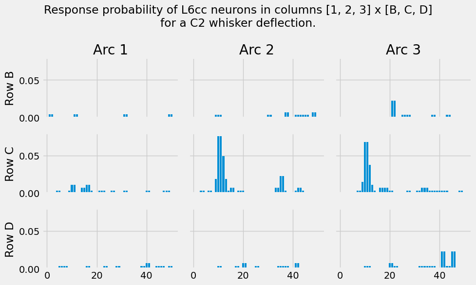
Ongoing activity
Ongoing activity is activity that does not depend on any kind of stimulus. ISF treats this as a special kind of activity source, modeled as Poisson spike trains.
[8]:
ongoing_data_dir = Path(getting_started_dir) / 'example_data' / 'functional_constraints' / 'ongoing_activity'
[9]:
I.plt.style.use("fivethirtyeight")
ongoing_rates = I.pd.read_csv(ongoing_data_dir / "measured_ongoing_rates.csv", sep='\t')
ongoing_rates.set_index("Cell type").plot.barh(figsize=(6, 8));
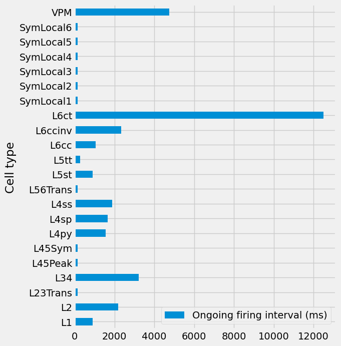
We can see that ongoing activity is defined in terms of average interval (in \(ms\)) for each cell type.
Important for later: there is no distinction between where these cells are located. Ongoing activity is expected to be the same across cells of the same cell type, independent of where they are located.
Synapse dynamics
We provide some default synapse dynamics models for glutamate and GABA receptors.
[10]:
exc_syn_fn = Path(getting_started_dir) / "example_data" / "functional_constraints" / "exc_synapse_template.param"
I.scp.build_parameters(exc_syn_fn).as_dict()
[10]:
{'synapses': {'receptors': {'glutamate_syn': {'threshold': 0.0,
    'delay': 0.0,
    'parameter': {'tau1': 26.0,
     'tau2': 2.0,
     'tau3': 2.0,
     'tau4': 0.1,
     'decayampa': 1.0,
     'decaynmda': 1.0},
    'weight': [1.0, 1.0]}},
  'releaseProb': 0.6}}
Adding activity data to network parameters
Network parameter files contain cell type-specific information on the following:
The network embedding (see the previous tutorial)
Synapse dynamics
Network activity (ongoing and/or evoked)
Here, we use NetworkParameterBuilder to add each component to a single cohesive parameter file. You could do this in a single line of code, but we will instead add each component one by one to inspect and explain the intermediate results.
The initial parameter object is empty, except for some auto-inferred info
[11]:
from singlecell_input_mapper.network_param_builder import NetworkParamBuilder

new_netp = NetworkParamBuilder().network_parameters
new_netp.as_dict()
[11]:
{'info': {'date': '2026-03-19', 'name': 'meulemeester'},
 'network': {},
 'NMODL_mechanisms': {}}
Adding ongoing activity
[12]:
celltype_to_ongoing_map = dict(
    zip(ongoing_rates['Cell type'], ongoing_rates['Ongoing firing interval (ms)'])
)

new_netp = NetworkParamBuilder(new_netp).add_ongoing_activity(
    # Mapping between cell type and ongoing interval in ms
    ongoing_interval_per_ct = celltype_to_ongoing_map

).network_parameters

new_netp.as_dict()
[12]:
{'info': {'date': '2026-03-19', 'name': 'meulemeester'},
 'network': {'L1': {'celltype': {'spiketrain': {'interval': 909.1}}},
  'L2': {'celltype': {'spiketrain': {'interval': 2173.9}}},
  'L23Trans': {'celltype': {'spiketrain': {'interval': 142.9}}},
  'L34': {'celltype': {'spiketrain': {'interval': 3225.8}}},
  'L45Peak': {'celltype': {'spiketrain': {'interval': 142.9}}},
  'L45Sym': {'celltype': {'spiketrain': {'interval': 142.9}}},
  'L4py': {'celltype': {'spiketrain': {'interval': 1562.5}}},
  'L4sp': {'celltype': {'spiketrain': {'interval': 1666.7}}},
  'L4ss': {'celltype': {'spiketrain': {'interval': 1886.8}}},
  'L56Trans': {'celltype': {'spiketrain': {'interval': 142.9}}},
  'L5st': {'celltype': {'spiketrain': {'interval': 909.1}}},
  'L5tt': {'celltype': {'spiketrain': {'interval': 283.3}}},
  'L6cc': {'celltype': {'spiketrain': {'interval': 1052.6}}},
  'L6ccinv': {'celltype': {'spiketrain': {'interval': 2325.6}}},
  'L6ct': {'celltype': {'spiketrain': {'interval': 12500.0}}},
  'SymLocal1': {'celltype': {'spiketrain': {'interval': 142.9}}},
  'SymLocal2': {'celltype': {'spiketrain': {'interval': 142.9}}},
  'SymLocal3': {'celltype': {'spiketrain': {'interval': 142.9}}},
  'SymLocal4': {'celltype': {'spiketrain': {'interval': 142.9}}},
  'SymLocal5': {'celltype': {'spiketrain': {'interval': 142.9}}},
  'SymLocal6': {'celltype': {'spiketrain': {'interval': 142.9}}},
  'VPM': {'celltype': {'spiketrain': {'interval': 4761.9}}}},
 'NMODL_mechanisms': {}}
Adding synapse dynamics
To add synapse dynamics, you could provide a mapping from cell type to specific synapse parameters. However, for this tutorial, we will simply assign generic excitatory and inhibitory synapses, depending on the cell type. This is the default fallback behavior of the NetworkParameterBuilder. Which cell types are excitatory or inhibitory should be configured in ISF’s user configuration, located in the config directory.
[13]:
new_netp = NetworkParamBuilder(new_netp).add_synapse_dynamics(
).network_parameters

new_netp.as_dict()
[WARNING] network_param_builder: No cell type specific synapse dynamics passed. Using generic synapse dynamics for excitatory and inhibitory instead. These can be configured in the user config.
[13]:
{'info': {'date': '2026-03-19', 'name': 'meulemeester'},
 'network': {'L1': {'celltype': {'spiketrain': {'interval': 909.1}},
   'synapses': {'receptors': {'gaba_syn': {'threshold': 0.0,
      'delay': 0.0,
      'parameter': {'decaygaba': 1.0,
       'risetime': 1.0,
       'decaytime': 20.0,
       'facilgaba': 0.0,
       'e': -80.0},
      'weight': 1.0}},
    'releaseProb': 0.25}},
  'L2': {'celltype': {'spiketrain': {'interval': 2173.9}},
   'synapses': {'receptors': {'glutamate_syn': {'threshold': 0.0,
      'delay': 0.0,
      'parameter': {'tau1': 26.0,
       'tau2': 2.0,
       'tau3': 2.0,
       'tau4': 0.1,
       'decayampa': 1.0,
       'decaynmda': 1.0},
      'weight': [1.0, 1.0]}},
    'releaseProb': 0.6}},
  'L23Trans': {'celltype': {'spiketrain': {'interval': 142.9}},
   'synapses': {'receptors': {'gaba_syn': {'threshold': 0.0,
      'delay': 0.0,
      'parameter': {'decaygaba': 1.0,
       'risetime': 1.0,
       'decaytime': 20.0,
       'facilgaba': 0.0,
       'e': -80.0},
      'weight': 1.0}},
    'releaseProb': 0.25}},
  'L34': {'celltype': {'spiketrain': {'interval': 3225.8}},
   'synapses': {'receptors': {'glutamate_syn': {'threshold': 0.0,
      'delay': 0.0,
      'parameter': {'tau1': 26.0,
       'tau2': 2.0,
       'tau3': 2.0,
       'tau4': 0.1,
       'decayampa': 1.0,
       'decaynmda': 1.0},
      'weight': [1.0, 1.0]}},
    'releaseProb': 0.6}},
  'L45Peak': {'celltype': {'spiketrain': {'interval': 142.9}},
   'synapses': {'receptors': {'gaba_syn': {'threshold': 0.0,
      'delay': 0.0,
      'parameter': {'decaygaba': 1.0,
       'risetime': 1.0,
       'decaytime': 20.0,
       'facilgaba': 0.0,
       'e': -80.0},
      'weight': 1.0}},
    'releaseProb': 0.25}},
  'L45Sym': {'celltype': {'spiketrain': {'interval': 142.9}},
   'synapses': {'receptors': {'gaba_syn': {'threshold': 0.0,
      'delay': 0.0,
      'parameter': {'decaygaba': 1.0,
       'risetime': 1.0,
       'decaytime': 20.0,
       'facilgaba': 0.0,
       'e': -80.0},
      'weight': 1.0}},
    'releaseProb': 0.25}},
  'L4py': {'celltype': {'spiketrain': {'interval': 1562.5}},
   'synapses': {'receptors': {'glutamate_syn': {'threshold': 0.0,
      'delay': 0.0,
      'parameter': {'tau1': 26.0,
       'tau2': 2.0,
       'tau3': 2.0,
       'tau4': 0.1,
       'decayampa': 1.0,
       'decaynmda': 1.0},
      'weight': [1.0, 1.0]}},
    'releaseProb': 0.6}},
  'L4sp': {'celltype': {'spiketrain': {'interval': 1666.7}},
   'synapses': {'receptors': {'glutamate_syn': {'threshold': 0.0,
      'delay': 0.0,
      'parameter': {'tau1': 26.0,
       'tau2': 2.0,
       'tau3': 2.0,
       'tau4': 0.1,
       'decayampa': 1.0,
       'decaynmda': 1.0},
      'weight': [1.0, 1.0]}},
    'releaseProb': 0.6}},
  'L4ss': {'celltype': {'spiketrain': {'interval': 1886.8}},
   'synapses': {'receptors': {'glutamate_syn': {'threshold': 0.0,
      'delay': 0.0,
      'parameter': {'tau1': 26.0,
       'tau2': 2.0,
       'tau3': 2.0,
       'tau4': 0.1,
       'decayampa': 1.0,
       'decaynmda': 1.0},
      'weight': [1.0, 1.0]}},
    'releaseProb': 0.6}},
  'L56Trans': {'celltype': {'spiketrain': {'interval': 142.9}},
   'synapses': {'receptors': {'gaba_syn': {'threshold': 0.0,
      'delay': 0.0,
      'parameter': {'decaygaba': 1.0,
       'risetime': 1.0,
       'decaytime': 20.0,
       'facilgaba': 0.0,
       'e': -80.0},
      'weight': 1.0}},
    'releaseProb': 0.25}},
  'L5st': {'celltype': {'spiketrain': {'interval': 909.1}},
   'synapses': {'receptors': {'glutamate_syn': {'threshold': 0.0,
      'delay': 0.0,
      'parameter': {'tau1': 26.0,
       'tau2': 2.0,
       'tau3': 2.0,
       'tau4': 0.1,
       'decayampa': 1.0,
       'decaynmda': 1.0},
      'weight': [1.0, 1.0]}},
    'releaseProb': 0.6}},
  'L5tt': {'celltype': {'spiketrain': {'interval': 283.3}},
   'synapses': {'receptors': {'glutamate_syn': {'threshold': 0.0,
      'delay': 0.0,
      'parameter': {'tau1': 26.0,
       'tau2': 2.0,
       'tau3': 2.0,
       'tau4': 0.1,
       'decayampa': 1.0,
       'decaynmda': 1.0},
      'weight': [1.0, 1.0]}},
    'releaseProb': 0.6}},
  'L6cc': {'celltype': {'spiketrain': {'interval': 1052.6}},
   'synapses': {'receptors': {'glutamate_syn': {'threshold': 0.0,
      'delay': 0.0,
      'parameter': {'tau1': 26.0,
       'tau2': 2.0,
       'tau3': 2.0,
       'tau4': 0.1,
       'decayampa': 1.0,
       'decaynmda': 1.0},
      'weight': [1.0, 1.0]}},
    'releaseProb': 0.6}},
  'L6ccinv': {'celltype': {'spiketrain': {'interval': 2325.6}},
   'synapses': {'receptors': {'glutamate_syn': {'threshold': 0.0,
      'delay': 0.0,
      'parameter': {'tau1': 26.0,
       'tau2': 2.0,
       'tau3': 2.0,
       'tau4': 0.1,
       'decayampa': 1.0,
       'decaynmda': 1.0},
      'weight': [1.0, 1.0]}},
    'releaseProb': 0.6}},
  'L6ct': {'celltype': {'spiketrain': {'interval': 12500.0}},
   'synapses': {'receptors': {'glutamate_syn': {'threshold': 0.0,
      'delay': 0.0,
      'parameter': {'tau1': 26.0,
       'tau2': 2.0,
       'tau3': 2.0,
       'tau4': 0.1,
       'decayampa': 1.0,
       'decaynmda': 1.0},
      'weight': [1.0, 1.0]}},
    'releaseProb': 0.6}},
  'SymLocal1': {'celltype': {'spiketrain': {'interval': 142.9}},
   'synapses': {'receptors': {'gaba_syn': {'threshold': 0.0,
      'delay': 0.0,
      'parameter': {'decaygaba': 1.0,
       'risetime': 1.0,
       'decaytime': 20.0,
       'facilgaba': 0.0,
       'e': -80.0},
      'weight': 1.0}},
    'releaseProb': 0.25}},
  'SymLocal2': {'celltype': {'spiketrain': {'interval': 142.9}},
   'synapses': {'receptors': {'gaba_syn': {'threshold': 0.0,
      'delay': 0.0,
      'parameter': {'decaygaba': 1.0,
       'risetime': 1.0,
       'decaytime': 20.0,
       'facilgaba': 0.0,
       'e': -80.0},
      'weight': 1.0}},
    'releaseProb': 0.25}},
  'SymLocal3': {'celltype': {'spiketrain': {'interval': 142.9}},
   'synapses': {'receptors': {'gaba_syn': {'threshold': 0.0,
      'delay': 0.0,
      'parameter': {'decaygaba': 1.0,
       'risetime': 1.0,
       'decaytime': 20.0,
       'facilgaba': 0.0,
       'e': -80.0},
      'weight': 1.0}},
    'releaseProb': 0.25}},
  'SymLocal4': {'celltype': {'spiketrain': {'interval': 142.9}},
   'synapses': {'receptors': {'gaba_syn': {'threshold': 0.0,
      'delay': 0.0,
      'parameter': {'decaygaba': 1.0,
       'risetime': 1.0,
       'decaytime': 20.0,
       'facilgaba': 0.0,
       'e': -80.0},
      'weight': 1.0}},
    'releaseProb': 0.25}},
  'SymLocal5': {'celltype': {'spiketrain': {'interval': 142.9}},
   'synapses': {'receptors': {'gaba_syn': {'threshold': 0.0,
      'delay': 0.0,
      'parameter': {'decaygaba': 1.0,
       'risetime': 1.0,
       'decaytime': 20.0,
       'facilgaba': 0.0,
       'e': -80.0},
      'weight': 1.0}},
    'releaseProb': 0.25}},
  'SymLocal6': {'celltype': {'spiketrain': {'interval': 142.9}},
   'synapses': {'receptors': {'gaba_syn': {'threshold': 0.0,
      'delay': 0.0,
      'parameter': {'decaygaba': 1.0,
       'risetime': 1.0,
       'decaytime': 20.0,
       'facilgaba': 0.0,
       'e': -80.0},
      'weight': 1.0}},
    'releaseProb': 0.25}},
  'VPM': {'celltype': {'spiketrain': {'interval': 4761.9}},
   'synapses': {'receptors': {'glutamate_syn': {'threshold': 0.0,
      'delay': 0.0,
      'parameter': {'tau1': 26.0,
       'tau2': 2.0,
       'tau3': 2.0,
       'tau4': 0.1,
       'decayampa': 1.0,
       'decaynmda': 1.0},
      'weight': [1.0, 1.0]}},
    'releaseProb': 0.6}}},
 'NMODL_mechanisms': {}}
Adding the network embedding
Note that network embedding data depends on the locations of each presynaptic cell:
[14]:
# This was built in the previous tutorial
# Make sure that you don't have multiple files in there
# Here, we assume they are unique and simply fetch the first one we find
network_embedding_db = I.DataBase(tutorial_output_dir)['network_modeling']

from singlecell_input_mapper.reader import read_nr_connected_cells_from_con
connected_cells = read_nr_connected_cells_from_con(
    network_embedding_db['anatomical_constraints'].get_file(".con")
)
connected_cells
[14]:
celltype
L1_B1         8
L1_B2        10
L1_B3         3
L1_Beta       2
L1_C1        15
             ..
VPM_C3        3
VPM_D1       10
VPM_D2        5
VPM_E1        5
VPM_Gamma     3
Length: 278, dtype: int64
To add this to our network parameters, we must first subcategorize it so it has the same cell types. We can split up existing cell types into more refined categories.
We could manually expand each cell type so it the network parameters specify info on all possible cell locations (e.g. split “L5tt” into “L5tt_A1”, “L5tt_A2” and so on). However, if a specific subcelltype makes no connection to our postsynaptic cell, it is of little use to define parameters for it. If it is not connected, we don’t care about it. We instead use the class method subcategorize_celltypes and give
it a mapping between cell types that already exist in the network parameters, and a list of subtypes. We infer this mapping from the cell types present in our `.con <>`__ file:
[15]:
subcategorized_celltypes_map= connected_cells.groupby(
    connected_cells.index.str.split("_").str[0]
).apply(
    lambda x: list(x.index)
).to_dict()
[16]:
new_netp = NetworkParamBuilder(new_netp).subcategorize_celltypes(
    cell_type_map = subcategorized_celltypes_map
).network_parameters

new_netp.as_dict()
[16]:
{'info': {'date': '2026-03-19', 'name': 'meulemeester'},
'network': {'L1_B1': {'celltype': {'spiketrain': {'interval': 909.1}},
'synapses': {'receptors': {'gaba_syn': {'threshold': 0.0,
'delay': 0.0,
'parameter': {'decaygaba': 1.0,
'risetime': 1.0,
'decaytime': 20.0,
'facilgaba': 0.0,
'e': -80.0},
'weight': 1.0}},
'releaseProb': 0.25}},
'L1_B2': {'celltype': {'spiketrain': {'interval': 909.1}},
'synapses': {'receptors': {'gaba_syn': {'threshold': 0.0,
'delay': 0.0,
'parameter': {'decaygaba': 1.0,
'risetime': 1.0,
'decaytime': 20.0,
'facilgaba': 0.0,
'e': -80.0},
'weight': 1.0}},
'releaseProb': 0.25}},
'L1_B3': {'celltype': {'spiketrain': {'interval': 909.1}},
'synapses': {'receptors': {'gaba_syn': {'threshold': 0.0,
'delay': 0.0,
'parameter': {'decaygaba': 1.0,
'risetime': 1.0,
'decaytime': 20.0,
'facilgaba': 0.0,
'e': -80.0},
'weight': 1.0}},
'releaseProb': 0.25}},
'L1_Beta': {'celltype': {'spiketrain': {'interval': 909.1}},
'synapses': {'receptors': {'gaba_syn': {'threshold': 0.0,
'delay': 0.0,
'parameter': {'decaygaba': 1.0,
'risetime': 1.0,
'decaytime': 20.0,
'facilgaba': 0.0,
'e': -80.0},
'weight': 1.0}},
'releaseProb': 0.25}},
'L1_C1': {'celltype': {'spiketrain': {'interval': 909.1}},
'synapses': {'receptors': {'gaba_syn': {'threshold': 0.0,
'delay': 0.0,
'parameter': {'decaygaba': 1.0,
'risetime': 1.0,
'decaytime': 20.0,
'facilgaba': 0.0,
'e': -80.0},
'weight': 1.0}},
'releaseProb': 0.25}},
'L1_C2': {'celltype': {'spiketrain': {'interval': 909.1}},
'synapses': {'receptors': {'gaba_syn': {'threshold': 0.0,
'delay': 0.0,
'parameter': {'decaygaba': 1.0,
'risetime': 1.0,
'decaytime': 20.0,
'facilgaba': 0.0,
'e': -80.0},
'weight': 1.0}},
'releaseProb': 0.25}},
'L1_C3': {'celltype': {'spiketrain': {'interval': 909.1}},
'synapses': {'receptors': {'gaba_syn': {'threshold': 0.0,
'delay': 0.0,
'parameter': {'decaygaba': 1.0,
'risetime': 1.0,
'decaytime': 20.0,
'facilgaba': 0.0,
'e': -80.0},
'weight': 1.0}},
'releaseProb': 0.25}},
'L1_D1': {'celltype': {'spiketrain': {'interval': 909.1}},
'synapses': {'receptors': {'gaba_syn': {'threshold': 0.0,
'delay': 0.0,
'parameter': {'decaygaba': 1.0,
'risetime': 1.0,
'decaytime': 20.0,
'facilgaba': 0.0,
'e': -80.0},
'weight': 1.0}},
'releaseProb': 0.25}},
'L1_D2': {'celltype': {'spiketrain': {'interval': 909.1}},
'synapses': {'receptors': {'gaba_syn': {'threshold': 0.0,
'delay': 0.0,
'parameter': {'decaygaba': 1.0,
'risetime': 1.0,
'decaytime': 20.0,
'facilgaba': 0.0,
'e': -80.0},
'weight': 1.0}},
'releaseProb': 0.25}},
'L1_D3': {'celltype': {'spiketrain': {'interval': 909.1}},
'synapses': {'receptors': {'gaba_syn': {'threshold': 0.0,
'delay': 0.0,
'parameter': {'decaygaba': 1.0,
'risetime': 1.0,
'decaytime': 20.0,
'facilgaba': 0.0,
'e': -80.0},
'weight': 1.0}},
'releaseProb': 0.25}},
'L1_E2': {'celltype': {'spiketrain': {'interval': 909.1}},
'synapses': {'receptors': {'gaba_syn': {'threshold': 0.0,
'delay': 0.0,
'parameter': {'decaygaba': 1.0,
'risetime': 1.0,
'decaytime': 20.0,
'facilgaba': 0.0,
'e': -80.0},
'weight': 1.0}},
'releaseProb': 0.25}},
'L2_Alpha': {'celltype': {'spiketrain': {'interval': 2173.9}},
'synapses': {'receptors': {'glutamate_syn': {'threshold': 0.0,
'delay': 0.0,
'parameter': {'tau1': 26.0,
'tau2': 2.0,
'tau3': 2.0,
'tau4': 0.1,
'decayampa': 1.0,
'decaynmda': 1.0},
'weight': [1.0, 1.0]}},
'releaseProb': 0.6}},
'L2_B1': {'celltype': {'spiketrain': {'interval': 2173.9}},
'synapses': {'receptors': {'glutamate_syn': {'threshold': 0.0,
'delay': 0.0,
'parameter': {'tau1': 26.0,
'tau2': 2.0,
'tau3': 2.0,
'tau4': 0.1,
'decayampa': 1.0,
'decaynmda': 1.0},
'weight': [1.0, 1.0]}},
'releaseProb': 0.6}},
'L2_B2': {'celltype': {'spiketrain': {'interval': 2173.9}},
'synapses': {'receptors': {'glutamate_syn': {'threshold': 0.0,
'delay': 0.0,
'parameter': {'tau1': 26.0,
'tau2': 2.0,
'tau3': 2.0,
'tau4': 0.1,
'decayampa': 1.0,
'decaynmda': 1.0},
'weight': [1.0, 1.0]}},
'releaseProb': 0.6}},
'L2_B3': {'celltype': {'spiketrain': {'interval': 2173.9}},
'synapses': {'receptors': {'glutamate_syn': {'threshold': 0.0,
'delay': 0.0,
'parameter': {'tau1': 26.0,
'tau2': 2.0,
'tau3': 2.0,
'tau4': 0.1,
'decayampa': 1.0,
'decaynmda': 1.0},
'weight': [1.0, 1.0]}},
'releaseProb': 0.6}},
'L2_B4': {'celltype': {'spiketrain': {'interval': 2173.9}},
'synapses': {'receptors': {'glutamate_syn': {'threshold': 0.0,
'delay': 0.0,
'parameter': {'tau1': 26.0,
'tau2': 2.0,
'tau3': 2.0,
'tau4': 0.1,
'decayampa': 1.0,
'decaynmda': 1.0},
'weight': [1.0, 1.0]}},
'releaseProb': 0.6}},
'L2_Beta': {'celltype': {'spiketrain': {'interval': 2173.9}},
'synapses': {'receptors': {'glutamate_syn': {'threshold': 0.0,
'delay': 0.0,
'parameter': {'tau1': 26.0,
'tau2': 2.0,
'tau3': 2.0,
'tau4': 0.1,
'decayampa': 1.0,
'decaynmda': 1.0},
'weight': [1.0, 1.0]}},
'releaseProb': 0.6}},
'L2_C1': {'celltype': {'spiketrain': {'interval': 2173.9}},
'synapses': {'receptors': {'glutamate_syn': {'threshold': 0.0,
'delay': 0.0,
'parameter': {'tau1': 26.0,
'tau2': 2.0,
'tau3': 2.0,
'tau4': 0.1,
'decayampa': 1.0,
'decaynmda': 1.0},
'weight': [1.0, 1.0]}},
'releaseProb': 0.6}},
'L2_C2': {'celltype': {'spiketrain': {'interval': 2173.9}},
'synapses': {'receptors': {'glutamate_syn': {'threshold': 0.0,
'delay': 0.0,
'parameter': {'tau1': 26.0,
'tau2': 2.0,
'tau3': 2.0,
'tau4': 0.1,
'decayampa': 1.0,
'decaynmda': 1.0},
'weight': [1.0, 1.0]}},
'releaseProb': 0.6}},
'L2_C3': {'celltype': {'spiketrain': {'interval': 2173.9}},
'synapses': {'receptors': {'glutamate_syn': {'threshold': 0.0,
'delay': 0.0,
'parameter': {'tau1': 26.0,
'tau2': 2.0,
'tau3': 2.0,
'tau4': 0.1,
'decayampa': 1.0,
'decaynmda': 1.0},
'weight': [1.0, 1.0]}},
'releaseProb': 0.6}},
'L2_C4': {'celltype': {'spiketrain': {'interval': 2173.9}},
'synapses': {'receptors': {'glutamate_syn': {'threshold': 0.0,
'delay': 0.0,
'parameter': {'tau1': 26.0,
'tau2': 2.0,
'tau3': 2.0,
'tau4': 0.1,
'decayampa': 1.0,
'decaynmda': 1.0},
'weight': [1.0, 1.0]}},
'releaseProb': 0.6}},
'L2_D1': {'celltype': {'spiketrain': {'interval': 2173.9}},
'synapses': {'receptors': {'glutamate_syn': {'threshold': 0.0,
'delay': 0.0,
'parameter': {'tau1': 26.0,
'tau2': 2.0,
'tau3': 2.0,
'tau4': 0.1,
'decayampa': 1.0,
'decaynmda': 1.0},
'weight': [1.0, 1.0]}},
'releaseProb': 0.6}},
'L2_D2': {'celltype': {'spiketrain': {'interval': 2173.9}},
'synapses': {'receptors': {'glutamate_syn': {'threshold': 0.0,
'delay': 0.0,
'parameter': {'tau1': 26.0,
'tau2': 2.0,
'tau3': 2.0,
'tau4': 0.1,
'decayampa': 1.0,
'decaynmda': 1.0},
'weight': [1.0, 1.0]}},
'releaseProb': 0.6}},
'L2_D3': {'celltype': {'spiketrain': {'interval': 2173.9}},
'synapses': {'receptors': {'glutamate_syn': {'threshold': 0.0,
'delay': 0.0,
'parameter': {'tau1': 26.0,
'tau2': 2.0,
'tau3': 2.0,
'tau4': 0.1,
'decayampa': 1.0,
'decaynmda': 1.0},
'weight': [1.0, 1.0]}},
'releaseProb': 0.6}},
'L2_D4': {'celltype': {'spiketrain': {'interval': 2173.9}},
'synapses': {'receptors': {'glutamate_syn': {'threshold': 0.0,
'delay': 0.0,
'parameter': {'tau1': 26.0,
'tau2': 2.0,
'tau3': 2.0,
'tau4': 0.1,
'decayampa': 1.0,
'decaynmda': 1.0},
'weight': [1.0, 1.0]}},
'releaseProb': 0.6}},
'L2_E1': {'celltype': {'spiketrain': {'interval': 2173.9}},
'synapses': {'receptors': {'glutamate_syn': {'threshold': 0.0,
'delay': 0.0,
'parameter': {'tau1': 26.0,
'tau2': 2.0,
'tau3': 2.0,
'tau4': 0.1,
'decayampa': 1.0,
'decaynmda': 1.0},
'weight': [1.0, 1.0]}},
'releaseProb': 0.6}},
'L2_E2': {'celltype': {'spiketrain': {'interval': 2173.9}},
'synapses': {'receptors': {'glutamate_syn': {'threshold': 0.0,
'delay': 0.0,
'parameter': {'tau1': 26.0,
'tau2': 2.0,
'tau3': 2.0,
'tau4': 0.1,
'decayampa': 1.0,
'decaynmda': 1.0},
'weight': [1.0, 1.0]}},
'releaseProb': 0.6}},
'L2_Gamma': {'celltype': {'spiketrain': {'interval': 2173.9}},
'synapses': {'receptors': {'glutamate_syn': {'threshold': 0.0,
'delay': 0.0,
'parameter': {'tau1': 26.0,
'tau2': 2.0,
'tau3': 2.0,
'tau4': 0.1,
'decayampa': 1.0,
'decaynmda': 1.0},
'weight': [1.0, 1.0]}},
'releaseProb': 0.6}},
'L23Trans_B1': {'celltype': {'spiketrain': {'interval': 142.9}},
'synapses': {'receptors': {'gaba_syn': {'threshold': 0.0,
'delay': 0.0,
'parameter': {'decaygaba': 1.0,
'risetime': 1.0,
'decaytime': 20.0,
'facilgaba': 0.0,
'e': -80.0},
'weight': 1.0}},
'releaseProb': 0.25}},
'L23Trans_B2': {'celltype': {'spiketrain': {'interval': 142.9}},
'synapses': {'receptors': {'gaba_syn': {'threshold': 0.0,
'delay': 0.0,
'parameter': {'decaygaba': 1.0,
'risetime': 1.0,
'decaytime': 20.0,
'facilgaba': 0.0,
'e': -80.0},
'weight': 1.0}},
'releaseProb': 0.25}},
'L23Trans_B3': {'celltype': {'spiketrain': {'interval': 142.9}},
'synapses': {'receptors': {'gaba_syn': {'threshold': 0.0,
'delay': 0.0,
'parameter': {'decaygaba': 1.0,
'risetime': 1.0,
'decaytime': 20.0,
'facilgaba': 0.0,
'e': -80.0},
'weight': 1.0}},
'releaseProb': 0.25}},
'L23Trans_C1': {'celltype': {'spiketrain': {'interval': 142.9}},
'synapses': {'receptors': {'gaba_syn': {'threshold': 0.0,
'delay': 0.0,
'parameter': {'decaygaba': 1.0,
'risetime': 1.0,
'decaytime': 20.0,
'facilgaba': 0.0,
'e': -80.0},
'weight': 1.0}},
'releaseProb': 0.25}},
'L23Trans_C2': {'celltype': {'spiketrain': {'interval': 142.9}},
'synapses': {'receptors': {'gaba_syn': {'threshold': 0.0,
'delay': 0.0,
'parameter': {'decaygaba': 1.0,
'risetime': 1.0,
'decaytime': 20.0,
'facilgaba': 0.0,
'e': -80.0},
'weight': 1.0}},
'releaseProb': 0.25}},
'L23Trans_C3': {'celltype': {'spiketrain': {'interval': 142.9}},
'synapses': {'receptors': {'gaba_syn': {'threshold': 0.0,
'delay': 0.0,
'parameter': {'decaygaba': 1.0,
'risetime': 1.0,
'decaytime': 20.0,
'facilgaba': 0.0,
'e': -80.0},
'weight': 1.0}},
'releaseProb': 0.25}},
'L23Trans_D1': {'celltype': {'spiketrain': {'interval': 142.9}},
'synapses': {'receptors': {'gaba_syn': {'threshold': 0.0,
'delay': 0.0,
'parameter': {'decaygaba': 1.0,
'risetime': 1.0,
'decaytime': 20.0,
'facilgaba': 0.0,
'e': -80.0},
'weight': 1.0}},
'releaseProb': 0.25}},
'L23Trans_D2': {'celltype': {'spiketrain': {'interval': 142.9}},
'synapses': {'receptors': {'gaba_syn': {'threshold': 0.0,
'delay': 0.0,
'parameter': {'decaygaba': 1.0,
'risetime': 1.0,
'decaytime': 20.0,
'facilgaba': 0.0,
'e': -80.0},
'weight': 1.0}},
'releaseProb': 0.25}},
'L34_A1': {'celltype': {'spiketrain': {'interval': 3225.8}},
'synapses': {'receptors': {'glutamate_syn': {'threshold': 0.0,
'delay': 0.0,
'parameter': {'tau1': 26.0,
'tau2': 2.0,
'tau3': 2.0,
'tau4': 0.1,
'decayampa': 1.0,
'decaynmda': 1.0},
'weight': [1.0, 1.0]}},
'releaseProb': 0.6}},
'L34_A2': {'celltype': {'spiketrain': {'interval': 3225.8}},
'synapses': {'receptors': {'glutamate_syn': {'threshold': 0.0,
'delay': 0.0,
'parameter': {'tau1': 26.0,
'tau2': 2.0,
'tau3': 2.0,
'tau4': 0.1,
'decayampa': 1.0,
'decaynmda': 1.0},
'weight': [1.0, 1.0]}},
'releaseProb': 0.6}},
'L34_A3': {'celltype': {'spiketrain': {'interval': 3225.8}},
'synapses': {'receptors': {'glutamate_syn': {'threshold': 0.0,
'delay': 0.0,
'parameter': {'tau1': 26.0,
'tau2': 2.0,
'tau3': 2.0,
'tau4': 0.1,
'decayampa': 1.0,
'decaynmda': 1.0},
'weight': [1.0, 1.0]}},
'releaseProb': 0.6}},
'L34_A4': {'celltype': {'spiketrain': {'interval': 3225.8}},
'synapses': {'receptors': {'glutamate_syn': {'threshold': 0.0,
'delay': 0.0,
'parameter': {'tau1': 26.0,
'tau2': 2.0,
'tau3': 2.0,
'tau4': 0.1,
'decayampa': 1.0,
'decaynmda': 1.0},
'weight': [1.0, 1.0]}},
'releaseProb': 0.6}},
'L34_Alpha': {'celltype': {'spiketrain': {'interval': 3225.8}},
'synapses': {'receptors': {'glutamate_syn': {'threshold': 0.0,
'delay': 0.0,
'parameter': {'tau1': 26.0,
'tau2': 2.0,
'tau3': 2.0,
'tau4': 0.1,
'decayampa': 1.0,
'decaynmda': 1.0},
'weight': [1.0, 1.0]}},
'releaseProb': 0.6}},
'L34_B1': {'celltype': {'spiketrain': {'interval': 3225.8}},
'synapses': {'receptors': {'glutamate_syn': {'threshold': 0.0,
'delay': 0.0,
'parameter': {'tau1': 26.0,
'tau2': 2.0,
'tau3': 2.0,
'tau4': 0.1,
'decayampa': 1.0,
'decaynmda': 1.0},
'weight': [1.0, 1.0]}},
'releaseProb': 0.6}},
'L34_B2': {'celltype': {'spiketrain': {'interval': 3225.8}},
'synapses': {'receptors': {'glutamate_syn': {'threshold': 0.0,
'delay': 0.0,
'parameter': {'tau1': 26.0,
'tau2': 2.0,
'tau3': 2.0,
'tau4': 0.1,
'decayampa': 1.0,
'decaynmda': 1.0},
'weight': [1.0, 1.0]}},
'releaseProb': 0.6}},
'L34_B3': {'celltype': {'spiketrain': {'interval': 3225.8}},
'synapses': {'receptors': {'glutamate_syn': {'threshold': 0.0,
'delay': 0.0,
'parameter': {'tau1': 26.0,
'tau2': 2.0,
'tau3': 2.0,
'tau4': 0.1,
'decayampa': 1.0,
'decaynmda': 1.0},
'weight': [1.0, 1.0]}},
'releaseProb': 0.6}},
'L34_B4': {'celltype': {'spiketrain': {'interval': 3225.8}},
'synapses': {'receptors': {'glutamate_syn': {'threshold': 0.0,
'delay': 0.0,
'parameter': {'tau1': 26.0,
'tau2': 2.0,
'tau3': 2.0,
'tau4': 0.1,
'decayampa': 1.0,
'decaynmda': 1.0},
'weight': [1.0, 1.0]}},
'releaseProb': 0.6}},
'L34_Beta': {'celltype': {'spiketrain': {'interval': 3225.8}},
'synapses': {'receptors': {'glutamate_syn': {'threshold': 0.0,
'delay': 0.0,
'parameter': {'tau1': 26.0,
'tau2': 2.0,
'tau3': 2.0,
'tau4': 0.1,
'decayampa': 1.0,
'decaynmda': 1.0},
'weight': [1.0, 1.0]}},
'releaseProb': 0.6}},
'L34_C1': {'celltype': {'spiketrain': {'interval': 3225.8}},
'synapses': {'receptors': {'glutamate_syn': {'threshold': 0.0,
'delay': 0.0,
'parameter': {'tau1': 26.0,
'tau2': 2.0,
'tau3': 2.0,
'tau4': 0.1,
'decayampa': 1.0,
'decaynmda': 1.0},
'weight': [1.0, 1.0]}},
'releaseProb': 0.6}},
'L34_C2': {'celltype': {'spiketrain': {'interval': 3225.8}},
'synapses': {'receptors': {'glutamate_syn': {'threshold': 0.0,
'delay': 0.0,
'parameter': {'tau1': 26.0,
'tau2': 2.0,
'tau3': 2.0,
'tau4': 0.1,
'decayampa': 1.0,
'decaynmda': 1.0},
'weight': [1.0, 1.0]}},
'releaseProb': 0.6}},
'L34_C3': {'celltype': {'spiketrain': {'interval': 3225.8}},
'synapses': {'receptors': {'glutamate_syn': {'threshold': 0.0,
'delay': 0.0,
'parameter': {'tau1': 26.0,
'tau2': 2.0,
'tau3': 2.0,
'tau4': 0.1,
'decayampa': 1.0,
'decaynmda': 1.0},
'weight': [1.0, 1.0]}},
'releaseProb': 0.6}},
'L34_C4': {'celltype': {'spiketrain': {'interval': 3225.8}},
'synapses': {'receptors': {'glutamate_syn': {'threshold': 0.0,
'delay': 0.0,
'parameter': {'tau1': 26.0,
'tau2': 2.0,
'tau3': 2.0,
'tau4': 0.1,
'decayampa': 1.0,
'decaynmda': 1.0},
'weight': [1.0, 1.0]}},
'releaseProb': 0.6}},
'L34_D1': {'celltype': {'spiketrain': {'interval': 3225.8}},
'synapses': {'receptors': {'glutamate_syn': {'threshold': 0.0,
'delay': 0.0,
'parameter': {'tau1': 26.0,
'tau2': 2.0,
'tau3': 2.0,
'tau4': 0.1,
'decayampa': 1.0,
'decaynmda': 1.0},
'weight': [1.0, 1.0]}},
'releaseProb': 0.6}},
'L34_D2': {'celltype': {'spiketrain': {'interval': 3225.8}},
'synapses': {'receptors': {'glutamate_syn': {'threshold': 0.0,
'delay': 0.0,
'parameter': {'tau1': 26.0,
'tau2': 2.0,
'tau3': 2.0,
'tau4': 0.1,
'decayampa': 1.0,
'decaynmda': 1.0},
'weight': [1.0, 1.0]}},
'releaseProb': 0.6}},
'L34_D3': {'celltype': {'spiketrain': {'interval': 3225.8}},
'synapses': {'receptors': {'glutamate_syn': {'threshold': 0.0,
'delay': 0.0,
'parameter': {'tau1': 26.0,
'tau2': 2.0,
'tau3': 2.0,
'tau4': 0.1,
'decayampa': 1.0,
'decaynmda': 1.0},
'weight': [1.0, 1.0]}},
'releaseProb': 0.6}},
'L34_Delta': {'celltype': {'spiketrain': {'interval': 3225.8}},
'synapses': {'receptors': {'glutamate_syn': {'threshold': 0.0,
'delay': 0.0,
'parameter': {'tau1': 26.0,
'tau2': 2.0,
'tau3': 2.0,
'tau4': 0.1,
'decayampa': 1.0,
'decaynmda': 1.0},
'weight': [1.0, 1.0]}},
'releaseProb': 0.6}},
'L34_E1': {'celltype': {'spiketrain': {'interval': 3225.8}},
'synapses': {'receptors': {'glutamate_syn': {'threshold': 0.0,
'delay': 0.0,
'parameter': {'tau1': 26.0,
'tau2': 2.0,
'tau3': 2.0,
'tau4': 0.1,
'decayampa': 1.0,
'decaynmda': 1.0},
'weight': [1.0, 1.0]}},
'releaseProb': 0.6}},
'L34_E2': {'celltype': {'spiketrain': {'interval': 3225.8}},
'synapses': {'receptors': {'glutamate_syn': {'threshold': 0.0,
'delay': 0.0,
'parameter': {'tau1': 26.0,
'tau2': 2.0,
'tau3': 2.0,
'tau4': 0.1,
'decayampa': 1.0,
'decaynmda': 1.0},
'weight': [1.0, 1.0]}},
'releaseProb': 0.6}},
'L34_E3': {'celltype': {'spiketrain': {'interval': 3225.8}},
'synapses': {'receptors': {'glutamate_syn': {'threshold': 0.0,
'delay': 0.0,
'parameter': {'tau1': 26.0,
'tau2': 2.0,
'tau3': 2.0,
'tau4': 0.1,
'decayampa': 1.0,
'decaynmda': 1.0},
'weight': [1.0, 1.0]}},
'releaseProb': 0.6}},
'L34_Gamma': {'celltype': {'spiketrain': {'interval': 3225.8}},
'synapses': {'receptors': {'glutamate_syn': {'threshold': 0.0,
'delay': 0.0,
'parameter': {'tau1': 26.0,
'tau2': 2.0,
'tau3': 2.0,
'tau4': 0.1,
'decayampa': 1.0,
'decaynmda': 1.0},
'weight': [1.0, 1.0]}},
'releaseProb': 0.6}},
'L45Peak_A2': {'celltype': {'spiketrain': {'interval': 142.9}},
'synapses': {'receptors': {'gaba_syn': {'threshold': 0.0,
'delay': 0.0,
'parameter': {'decaygaba': 1.0,
'risetime': 1.0,
'decaytime': 20.0,
'facilgaba': 0.0,
'e': -80.0},
'weight': 1.0}},
'releaseProb': 0.25}},
'L45Peak_A4': {'celltype': {'spiketrain': {'interval': 142.9}},
'synapses': {'receptors': {'gaba_syn': {'threshold': 0.0,
'delay': 0.0,
'parameter': {'decaygaba': 1.0,
'risetime': 1.0,
'decaytime': 20.0,
'facilgaba': 0.0,
'e': -80.0},
'weight': 1.0}},
'releaseProb': 0.25}},
'L45Peak_B1': {'celltype': {'spiketrain': {'interval': 142.9}},
'synapses': {'receptors': {'gaba_syn': {'threshold': 0.0,
'delay': 0.0,
'parameter': {'decaygaba': 1.0,
'risetime': 1.0,
'decaytime': 20.0,
'facilgaba': 0.0,
'e': -80.0},
'weight': 1.0}},
'releaseProb': 0.25}},
'L45Peak_B2': {'celltype': {'spiketrain': {'interval': 142.9}},
'synapses': {'receptors': {'gaba_syn': {'threshold': 0.0,
'delay': 0.0,
'parameter': {'decaygaba': 1.0,
'risetime': 1.0,
'decaytime': 20.0,
'facilgaba': 0.0,
'e': -80.0},
'weight': 1.0}},
'releaseProb': 0.25}},
'L45Peak_B3': {'celltype': {'spiketrain': {'interval': 142.9}},
'synapses': {'receptors': {'gaba_syn': {'threshold': 0.0,
'delay': 0.0,
'parameter': {'decaygaba': 1.0,
'risetime': 1.0,
'decaytime': 20.0,
'facilgaba': 0.0,
'e': -80.0},
'weight': 1.0}},
'releaseProb': 0.25}},
'L45Peak_B4': {'celltype': {'spiketrain': {'interval': 142.9}},
'synapses': {'receptors': {'gaba_syn': {'threshold': 0.0,
'delay': 0.0,
'parameter': {'decaygaba': 1.0,
'risetime': 1.0,
'decaytime': 20.0,
'facilgaba': 0.0,
'e': -80.0},
'weight': 1.0}},
'releaseProb': 0.25}},
'L45Peak_C1': {'celltype': {'spiketrain': {'interval': 142.9}},
'synapses': {'receptors': {'gaba_syn': {'threshold': 0.0,
'delay': 0.0,
'parameter': {'decaygaba': 1.0,
'risetime': 1.0,
'decaytime': 20.0,
'facilgaba': 0.0,
'e': -80.0},
'weight': 1.0}},
'releaseProb': 0.25}},
'L45Peak_C2': {'celltype': {'spiketrain': {'interval': 142.9}},
'synapses': {'receptors': {'gaba_syn': {'threshold': 0.0,
'delay': 0.0,
'parameter': {'decaygaba': 1.0,
'risetime': 1.0,
'decaytime': 20.0,
'facilgaba': 0.0,
'e': -80.0},
'weight': 1.0}},
'releaseProb': 0.25}},
'L45Peak_C3': {'celltype': {'spiketrain': {'interval': 142.9}},
'synapses': {'receptors': {'gaba_syn': {'threshold': 0.0,
'delay': 0.0,
'parameter': {'decaygaba': 1.0,
'risetime': 1.0,
'decaytime': 20.0,
'facilgaba': 0.0,
'e': -80.0},
'weight': 1.0}},
'releaseProb': 0.25}},
'L45Peak_D1': {'celltype': {'spiketrain': {'interval': 142.9}},
'synapses': {'receptors': {'gaba_syn': {'threshold': 0.0,
'delay': 0.0,
'parameter': {'decaygaba': 1.0,
'risetime': 1.0,
'decaytime': 20.0,
'facilgaba': 0.0,
'e': -80.0},
'weight': 1.0}},
'releaseProb': 0.25}},
'L45Peak_D2': {'celltype': {'spiketrain': {'interval': 142.9}},
'synapses': {'receptors': {'gaba_syn': {'threshold': 0.0,
'delay': 0.0,
'parameter': {'decaygaba': 1.0,
'risetime': 1.0,
'decaytime': 20.0,
'facilgaba': 0.0,
'e': -80.0},
'weight': 1.0}},
'releaseProb': 0.25}},
'L45Peak_Delta': {'celltype': {'spiketrain': {'interval': 142.9}},
'synapses': {'receptors': {'gaba_syn': {'threshold': 0.0,
'delay': 0.0,
'parameter': {'decaygaba': 1.0,
'risetime': 1.0,
'decaytime': 20.0,
'facilgaba': 0.0,
'e': -80.0},
'weight': 1.0}},
'releaseProb': 0.25}},
'L45Peak_Gamma': {'celltype': {'spiketrain': {'interval': 142.9}},
'synapses': {'receptors': {'gaba_syn': {'threshold': 0.0,
'delay': 0.0,
'parameter': {'decaygaba': 1.0,
'risetime': 1.0,
'decaytime': 20.0,
'facilgaba': 0.0,
'e': -80.0},
'weight': 1.0}},
'releaseProb': 0.25}},
'L45Sym_A3': {'celltype': {'spiketrain': {'interval': 142.9}},
'synapses': {'receptors': {'gaba_syn': {'threshold': 0.0,
'delay': 0.0,
'parameter': {'decaygaba': 1.0,
'risetime': 1.0,
'decaytime': 20.0,
'facilgaba': 0.0,
'e': -80.0},
'weight': 1.0}},
'releaseProb': 0.25}},
'L45Sym_B1': {'celltype': {'spiketrain': {'interval': 142.9}},
'synapses': {'receptors': {'gaba_syn': {'threshold': 0.0,
'delay': 0.0,
'parameter': {'decaygaba': 1.0,
'risetime': 1.0,
'decaytime': 20.0,
'facilgaba': 0.0,
'e': -80.0},
'weight': 1.0}},
'releaseProb': 0.25}},
'L45Sym_B2': {'celltype': {'spiketrain': {'interval': 142.9}},
'synapses': {'receptors': {'gaba_syn': {'threshold': 0.0,
'delay': 0.0,
'parameter': {'decaygaba': 1.0,
'risetime': 1.0,
'decaytime': 20.0,
'facilgaba': 0.0,
'e': -80.0},
'weight': 1.0}},
'releaseProb': 0.25}},
'L45Sym_B3': {'celltype': {'spiketrain': {'interval': 142.9}},
'synapses': {'receptors': {'gaba_syn': {'threshold': 0.0,
'delay': 0.0,
'parameter': {'decaygaba': 1.0,
'risetime': 1.0,
'decaytime': 20.0,
'facilgaba': 0.0,
'e': -80.0},
'weight': 1.0}},
'releaseProb': 0.25}},
'L45Sym_C1': {'celltype': {'spiketrain': {'interval': 142.9}},
'synapses': {'receptors': {'gaba_syn': {'threshold': 0.0,
'delay': 0.0,
'parameter': {'decaygaba': 1.0,
'risetime': 1.0,
'decaytime': 20.0,
'facilgaba': 0.0,
'e': -80.0},
'weight': 1.0}},
'releaseProb': 0.25}},
'L45Sym_C2': {'celltype': {'spiketrain': {'interval': 142.9}},
'synapses': {'receptors': {'gaba_syn': {'threshold': 0.0,
'delay': 0.0,
'parameter': {'decaygaba': 1.0,
'risetime': 1.0,
'decaytime': 20.0,
'facilgaba': 0.0,
'e': -80.0},
'weight': 1.0}},
'releaseProb': 0.25}},
'L45Sym_C3': {'celltype': {'spiketrain': {'interval': 142.9}},
'synapses': {'receptors': {'gaba_syn': {'threshold': 0.0,
'delay': 0.0,
'parameter': {'decaygaba': 1.0,
'risetime': 1.0,
'decaytime': 20.0,
'facilgaba': 0.0,
'e': -80.0},
'weight': 1.0}},
'releaseProb': 0.25}},
'L45Sym_D1': {'celltype': {'spiketrain': {'interval': 142.9}},
'synapses': {'receptors': {'gaba_syn': {'threshold': 0.0,
'delay': 0.0,
'parameter': {'decaygaba': 1.0,
'risetime': 1.0,
'decaytime': 20.0,
'facilgaba': 0.0,
'e': -80.0},
'weight': 1.0}},
'releaseProb': 0.25}},
'L45Sym_D2': {'celltype': {'spiketrain': {'interval': 142.9}},
'synapses': {'receptors': {'gaba_syn': {'threshold': 0.0,
'delay': 0.0,
'parameter': {'decaygaba': 1.0,
'risetime': 1.0,
'decaytime': 20.0,
'facilgaba': 0.0,
'e': -80.0},
'weight': 1.0}},
'releaseProb': 0.25}},
'L45Sym_E1': {'celltype': {'spiketrain': {'interval': 142.9}},
'synapses': {'receptors': {'gaba_syn': {'threshold': 0.0,
'delay': 0.0,
'parameter': {'decaygaba': 1.0,
'risetime': 1.0,
'decaytime': 20.0,
'facilgaba': 0.0,
'e': -80.0},
'weight': 1.0}},
'releaseProb': 0.25}},
'L4py_A1': {'celltype': {'spiketrain': {'interval': 1562.5}},
'synapses': {'receptors': {'glutamate_syn': {'threshold': 0.0,
'delay': 0.0,
'parameter': {'tau1': 26.0,
'tau2': 2.0,
'tau3': 2.0,
'tau4': 0.1,
'decayampa': 1.0,
'decaynmda': 1.0},
'weight': [1.0, 1.0]}},
'releaseProb': 0.6}},
'L4py_A2': {'celltype': {'spiketrain': {'interval': 1562.5}},
'synapses': {'receptors': {'glutamate_syn': {'threshold': 0.0,
'delay': 0.0,
'parameter': {'tau1': 26.0,
'tau2': 2.0,
'tau3': 2.0,
'tau4': 0.1,
'decayampa': 1.0,
'decaynmda': 1.0},
'weight': [1.0, 1.0]}},
'releaseProb': 0.6}},
'L4py_A3': {'celltype': {'spiketrain': {'interval': 1562.5}},
'synapses': {'receptors': {'glutamate_syn': {'threshold': 0.0,
'delay': 0.0,
'parameter': {'tau1': 26.0,
'tau2': 2.0,
'tau3': 2.0,
'tau4': 0.1,
'decayampa': 1.0,
'decaynmda': 1.0},
'weight': [1.0, 1.0]}},
'releaseProb': 0.6}},
'L4py_A4': {'celltype': {'spiketrain': {'interval': 1562.5}},
'synapses': {'receptors': {'glutamate_syn': {'threshold': 0.0,
'delay': 0.0,
'parameter': {'tau1': 26.0,
'tau2': 2.0,
'tau3': 2.0,
'tau4': 0.1,
'decayampa': 1.0,
'decaynmda': 1.0},
'weight': [1.0, 1.0]}},
'releaseProb': 0.6}},
'L4py_Alpha': {'celltype': {'spiketrain': {'interval': 1562.5}},
'synapses': {'receptors': {'glutamate_syn': {'threshold': 0.0,
'delay': 0.0,
'parameter': {'tau1': 26.0,
'tau2': 2.0,
'tau3': 2.0,
'tau4': 0.1,
'decayampa': 1.0,
'decaynmda': 1.0},
'weight': [1.0, 1.0]}},
'releaseProb': 0.6}},
'L4py_B1': {'celltype': {'spiketrain': {'interval': 1562.5}},
'synapses': {'receptors': {'glutamate_syn': {'threshold': 0.0,
'delay': 0.0,
'parameter': {'tau1': 26.0,
'tau2': 2.0,
'tau3': 2.0,
'tau4': 0.1,
'decayampa': 1.0,
'decaynmda': 1.0},
'weight': [1.0, 1.0]}},
'releaseProb': 0.6}},
'L4py_B2': {'celltype': {'spiketrain': {'interval': 1562.5}},
'synapses': {'receptors': {'glutamate_syn': {'threshold': 0.0,
'delay': 0.0,
'parameter': {'tau1': 26.0,
'tau2': 2.0,
'tau3': 2.0,
'tau4': 0.1,
'decayampa': 1.0,
'decaynmda': 1.0},
'weight': [1.0, 1.0]}},
'releaseProb': 0.6}},
'L4py_B3': {'celltype': {'spiketrain': {'interval': 1562.5}},
'synapses': {'receptors': {'glutamate_syn': {'threshold': 0.0,
'delay': 0.0,
'parameter': {'tau1': 26.0,
'tau2': 2.0,
'tau3': 2.0,
'tau4': 0.1,
'decayampa': 1.0,
'decaynmda': 1.0},
'weight': [1.0, 1.0]}},
'releaseProb': 0.6}},
'L4py_B4': {'celltype': {'spiketrain': {'interval': 1562.5}},
'synapses': {'receptors': {'glutamate_syn': {'threshold': 0.0,
'delay': 0.0,
'parameter': {'tau1': 26.0,
'tau2': 2.0,
'tau3': 2.0,
'tau4': 0.1,
'decayampa': 1.0,
'decaynmda': 1.0},
'weight': [1.0, 1.0]}},
'releaseProb': 0.6}},
'L4py_C1': {'celltype': {'spiketrain': {'interval': 1562.5}},
'synapses': {'receptors': {'glutamate_syn': {'threshold': 0.0,
'delay': 0.0,
'parameter': {'tau1': 26.0,
'tau2': 2.0,
'tau3': 2.0,
'tau4': 0.1,
'decayampa': 1.0,
'decaynmda': 1.0},
'weight': [1.0, 1.0]}},
'releaseProb': 0.6}},
'L4py_C2': {'celltype': {'spiketrain': {'interval': 1562.5}},
'synapses': {'receptors': {'glutamate_syn': {'threshold': 0.0,
'delay': 0.0,
'parameter': {'tau1': 26.0,
'tau2': 2.0,
'tau3': 2.0,
'tau4': 0.1,
'decayampa': 1.0,
'decaynmda': 1.0},
'weight': [1.0, 1.0]}},
'releaseProb': 0.6}},
'L4py_C3': {'celltype': {'spiketrain': {'interval': 1562.5}},
'synapses': {'receptors': {'glutamate_syn': {'threshold': 0.0,
'delay': 0.0,
'parameter': {'tau1': 26.0,
'tau2': 2.0,
'tau3': 2.0,
'tau4': 0.1,
'decayampa': 1.0,
'decaynmda': 1.0},
'weight': [1.0, 1.0]}},
'releaseProb': 0.6}},
'L4py_C4': {'celltype': {'spiketrain': {'interval': 1562.5}},
'synapses': {'receptors': {'glutamate_syn': {'threshold': 0.0,
'delay': 0.0,
'parameter': {'tau1': 26.0,
'tau2': 2.0,
'tau3': 2.0,
'tau4': 0.1,
'decayampa': 1.0,
'decaynmda': 1.0},
'weight': [1.0, 1.0]}},
'releaseProb': 0.6}},
'L4py_D1': {'celltype': {'spiketrain': {'interval': 1562.5}},
'synapses': {'receptors': {'glutamate_syn': {'threshold': 0.0,
'delay': 0.0,
'parameter': {'tau1': 26.0,
'tau2': 2.0,
'tau3': 2.0,
'tau4': 0.1,
'decayampa': 1.0,
'decaynmda': 1.0},
'weight': [1.0, 1.0]}},
'releaseProb': 0.6}},
'L4py_D2': {'celltype': {'spiketrain': {'interval': 1562.5}},
'synapses': {'receptors': {'glutamate_syn': {'threshold': 0.0,
'delay': 0.0,
'parameter': {'tau1': 26.0,
'tau2': 2.0,
'tau3': 2.0,
'tau4': 0.1,
'decayampa': 1.0,
'decaynmda': 1.0},
'weight': [1.0, 1.0]}},
'releaseProb': 0.6}},
'L4py_D3': {'celltype': {'spiketrain': {'interval': 1562.5}},
'synapses': {'receptors': {'glutamate_syn': {'threshold': 0.0,
'delay': 0.0,
'parameter': {'tau1': 26.0,
'tau2': 2.0,
'tau3': 2.0,
'tau4': 0.1,
'decayampa': 1.0,
'decaynmda': 1.0},
'weight': [1.0, 1.0]}},
'releaseProb': 0.6}},
'L4py_Gamma': {'celltype': {'spiketrain': {'interval': 1562.5}},
'synapses': {'receptors': {'glutamate_syn': {'threshold': 0.0,
'delay': 0.0,
'parameter': {'tau1': 26.0,
'tau2': 2.0,
'tau3': 2.0,
'tau4': 0.1,
'decayampa': 1.0,
'decaynmda': 1.0},
'weight': [1.0, 1.0]}},
'releaseProb': 0.6}},
'L4sp_B1': {'celltype': {'spiketrain': {'interval': 1666.7}},
'synapses': {'receptors': {'glutamate_syn': {'threshold': 0.0,
'delay': 0.0,
'parameter': {'tau1': 26.0,
'tau2': 2.0,
'tau3': 2.0,
'tau4': 0.1,
'decayampa': 1.0,
'decaynmda': 1.0},
'weight': [1.0, 1.0]}},
'releaseProb': 0.6}},
'L4sp_B2': {'celltype': {'spiketrain': {'interval': 1666.7}},
'synapses': {'receptors': {'glutamate_syn': {'threshold': 0.0,
'delay': 0.0,
'parameter': {'tau1': 26.0,
'tau2': 2.0,
'tau3': 2.0,
'tau4': 0.1,
'decayampa': 1.0,
'decaynmda': 1.0},
'weight': [1.0, 1.0]}},
'releaseProb': 0.6}},
'L4sp_B3': {'celltype': {'spiketrain': {'interval': 1666.7}},
'synapses': {'receptors': {'glutamate_syn': {'threshold': 0.0,
'delay': 0.0,
'parameter': {'tau1': 26.0,
'tau2': 2.0,
'tau3': 2.0,
'tau4': 0.1,
'decayampa': 1.0,
'decaynmda': 1.0},
'weight': [1.0, 1.0]}},
'releaseProb': 0.6}},
'L4sp_Beta': {'celltype': {'spiketrain': {'interval': 1666.7}},
'synapses': {'receptors': {'glutamate_syn': {'threshold': 0.0,
'delay': 0.0,
'parameter': {'tau1': 26.0,
'tau2': 2.0,
'tau3': 2.0,
'tau4': 0.1,
'decayampa': 1.0,
'decaynmda': 1.0},
'weight': [1.0, 1.0]}},
'releaseProb': 0.6}},
'L4sp_C1': {'celltype': {'spiketrain': {'interval': 1666.7}},
'synapses': {'receptors': {'glutamate_syn': {'threshold': 0.0,
'delay': 0.0,
'parameter': {'tau1': 26.0,
'tau2': 2.0,
'tau3': 2.0,
'tau4': 0.1,
'decayampa': 1.0,
'decaynmda': 1.0},
'weight': [1.0, 1.0]}},
'releaseProb': 0.6}},
'L4sp_C2': {'celltype': {'spiketrain': {'interval': 1666.7}},
'synapses': {'receptors': {'glutamate_syn': {'threshold': 0.0,
'delay': 0.0,
'parameter': {'tau1': 26.0,
'tau2': 2.0,
'tau3': 2.0,
'tau4': 0.1,
'decayampa': 1.0,
'decaynmda': 1.0},
'weight': [1.0, 1.0]}},
'releaseProb': 0.6}},
'L4sp_C3': {'celltype': {'spiketrain': {'interval': 1666.7}},
'synapses': {'receptors': {'glutamate_syn': {'threshold': 0.0,
'delay': 0.0,
'parameter': {'tau1': 26.0,
'tau2': 2.0,
'tau3': 2.0,
'tau4': 0.1,
'decayampa': 1.0,
'decaynmda': 1.0},
'weight': [1.0, 1.0]}},
'releaseProb': 0.6}},
'L4sp_C4': {'celltype': {'spiketrain': {'interval': 1666.7}},
'synapses': {'receptors': {'glutamate_syn': {'threshold': 0.0,
'delay': 0.0,
'parameter': {'tau1': 26.0,
'tau2': 2.0,
'tau3': 2.0,
'tau4': 0.1,
'decayampa': 1.0,
'decaynmda': 1.0},
'weight': [1.0, 1.0]}},
'releaseProb': 0.6}},
'L4sp_D1': {'celltype': {'spiketrain': {'interval': 1666.7}},
'synapses': {'receptors': {'glutamate_syn': {'threshold': 0.0,
'delay': 0.0,
'parameter': {'tau1': 26.0,
'tau2': 2.0,
'tau3': 2.0,
'tau4': 0.1,
'decayampa': 1.0,
'decaynmda': 1.0},
'weight': [1.0, 1.0]}},
'releaseProb': 0.6}},
'L4sp_D2': {'celltype': {'spiketrain': {'interval': 1666.7}},
'synapses': {'receptors': {'glutamate_syn': {'threshold': 0.0,
'delay': 0.0,
'parameter': {'tau1': 26.0,
'tau2': 2.0,
'tau3': 2.0,
'tau4': 0.1,
'decayampa': 1.0,
'decaynmda': 1.0},
'weight': [1.0, 1.0]}},
'releaseProb': 0.6}},
'L4sp_D3': {'celltype': {'spiketrain': {'interval': 1666.7}},
'synapses': {'receptors': {'glutamate_syn': {'threshold': 0.0,
'delay': 0.0,
'parameter': {'tau1': 26.0,
'tau2': 2.0,
'tau3': 2.0,
'tau4': 0.1,
'decayampa': 1.0,
'decaynmda': 1.0},
'weight': [1.0, 1.0]}},
'releaseProb': 0.6}},
'L4sp_Delta': {'celltype': {'spiketrain': {'interval': 1666.7}},
'synapses': {'receptors': {'glutamate_syn': {'threshold': 0.0,
'delay': 0.0,
'parameter': {'tau1': 26.0,
'tau2': 2.0,
'tau3': 2.0,
'tau4': 0.1,
'decayampa': 1.0,
'decaynmda': 1.0},
'weight': [1.0, 1.0]}},
'releaseProb': 0.6}},
'L4ss_A1': {'celltype': {'spiketrain': {'interval': 1886.8}},
'synapses': {'receptors': {'glutamate_syn': {'threshold': 0.0,
'delay': 0.0,
'parameter': {'tau1': 26.0,
'tau2': 2.0,
'tau3': 2.0,
'tau4': 0.1,
'decayampa': 1.0,
'decaynmda': 1.0},
'weight': [1.0, 1.0]}},
'releaseProb': 0.6}},
'L4ss_B1': {'celltype': {'spiketrain': {'interval': 1886.8}},
'synapses': {'receptors': {'glutamate_syn': {'threshold': 0.0,
'delay': 0.0,
'parameter': {'tau1': 26.0,
'tau2': 2.0,
'tau3': 2.0,
'tau4': 0.1,
'decayampa': 1.0,
'decaynmda': 1.0},
'weight': [1.0, 1.0]}},
'releaseProb': 0.6}},
'L4ss_B2': {'celltype': {'spiketrain': {'interval': 1886.8}},
'synapses': {'receptors': {'glutamate_syn': {'threshold': 0.0,
'delay': 0.0,
'parameter': {'tau1': 26.0,
'tau2': 2.0,
'tau3': 2.0,
'tau4': 0.1,
'decayampa': 1.0,
'decaynmda': 1.0},
'weight': [1.0, 1.0]}},
'releaseProb': 0.6}},
'L4ss_B3': {'celltype': {'spiketrain': {'interval': 1886.8}},
'synapses': {'receptors': {'glutamate_syn': {'threshold': 0.0,
'delay': 0.0,
'parameter': {'tau1': 26.0,
'tau2': 2.0,
'tau3': 2.0,
'tau4': 0.1,
'decayampa': 1.0,
'decaynmda': 1.0},
'weight': [1.0, 1.0]}},
'releaseProb': 0.6}},
'L4ss_C1': {'celltype': {'spiketrain': {'interval': 1886.8}},
'synapses': {'receptors': {'glutamate_syn': {'threshold': 0.0,
'delay': 0.0,
'parameter': {'tau1': 26.0,
'tau2': 2.0,
'tau3': 2.0,
'tau4': 0.1,
'decayampa': 1.0,
'decaynmda': 1.0},
'weight': [1.0, 1.0]}},
'releaseProb': 0.6}},
'L4ss_C2': {'celltype': {'spiketrain': {'interval': 1886.8}},
'synapses': {'receptors': {'glutamate_syn': {'threshold': 0.0,
'delay': 0.0,
'parameter': {'tau1': 26.0,
'tau2': 2.0,
'tau3': 2.0,
'tau4': 0.1,
'decayampa': 1.0,
'decaynmda': 1.0},
'weight': [1.0, 1.0]}},
'releaseProb': 0.6}},
'L4ss_C3': {'celltype': {'spiketrain': {'interval': 1886.8}},
'synapses': {'receptors': {'glutamate_syn': {'threshold': 0.0,
'delay': 0.0,
'parameter': {'tau1': 26.0,
'tau2': 2.0,
'tau3': 2.0,
'tau4': 0.1,
'decayampa': 1.0,
'decaynmda': 1.0},
'weight': [1.0, 1.0]}},
'releaseProb': 0.6}},
'L4ss_D1': {'celltype': {'spiketrain': {'interval': 1886.8}},
'synapses': {'receptors': {'glutamate_syn': {'threshold': 0.0,
'delay': 0.0,
'parameter': {'tau1': 26.0,
'tau2': 2.0,
'tau3': 2.0,
'tau4': 0.1,
'decayampa': 1.0,
'decaynmda': 1.0},
'weight': [1.0, 1.0]}},
'releaseProb': 0.6}},
'L4ss_D2': {'celltype': {'spiketrain': {'interval': 1886.8}},
'synapses': {'receptors': {'glutamate_syn': {'threshold': 0.0,
'delay': 0.0,
'parameter': {'tau1': 26.0,
'tau2': 2.0,
'tau3': 2.0,
'tau4': 0.1,
'decayampa': 1.0,
'decaynmda': 1.0},
'weight': [1.0, 1.0]}},
'releaseProb': 0.6}},
'L4ss_D3': {'celltype': {'spiketrain': {'interval': 1886.8}},
'synapses': {'receptors': {'glutamate_syn': {'threshold': 0.0,
'delay': 0.0,
'parameter': {'tau1': 26.0,
'tau2': 2.0,
'tau3': 2.0,
'tau4': 0.1,
'decayampa': 1.0,
'decaynmda': 1.0},
'weight': [1.0, 1.0]}},
'releaseProb': 0.6}},
'L4ss_E1': {'celltype': {'spiketrain': {'interval': 1886.8}},
'synapses': {'receptors': {'glutamate_syn': {'threshold': 0.0,
'delay': 0.0,
'parameter': {'tau1': 26.0,
'tau2': 2.0,
'tau3': 2.0,
'tau4': 0.1,
'decayampa': 1.0,
'decaynmda': 1.0},
'weight': [1.0, 1.0]}},
'releaseProb': 0.6}},
'L56Trans_A2': {'celltype': {'spiketrain': {'interval': 142.9}},
'synapses': {'receptors': {'gaba_syn': {'threshold': 0.0,
'delay': 0.0,
'parameter': {'decaygaba': 1.0,
'risetime': 1.0,
'decaytime': 20.0,
'facilgaba': 0.0,
'e': -80.0},
'weight': 1.0}},
'releaseProb': 0.25}},
'L56Trans_A3': {'celltype': {'spiketrain': {'interval': 142.9}},
'synapses': {'receptors': {'gaba_syn': {'threshold': 0.0,
'delay': 0.0,
'parameter': {'decaygaba': 1.0,
'risetime': 1.0,
'decaytime': 20.0,
'facilgaba': 0.0,
'e': -80.0},
'weight': 1.0}},
'releaseProb': 0.25}},
'L56Trans_A4': {'celltype': {'spiketrain': {'interval': 142.9}},
'synapses': {'receptors': {'gaba_syn': {'threshold': 0.0,
'delay': 0.0,
'parameter': {'decaygaba': 1.0,
'risetime': 1.0,
'decaytime': 20.0,
'facilgaba': 0.0,
'e': -80.0},
'weight': 1.0}},
'releaseProb': 0.25}},
'L56Trans_B1': {'celltype': {'spiketrain': {'interval': 142.9}},
'synapses': {'receptors': {'gaba_syn': {'threshold': 0.0,
'delay': 0.0,
'parameter': {'decaygaba': 1.0,
'risetime': 1.0,
'decaytime': 20.0,
'facilgaba': 0.0,
'e': -80.0},
'weight': 1.0}},
'releaseProb': 0.25}},
'L56Trans_B2': {'celltype': {'spiketrain': {'interval': 142.9}},
'synapses': {'receptors': {'gaba_syn': {'threshold': 0.0,
'delay': 0.0,
'parameter': {'decaygaba': 1.0,
'risetime': 1.0,
'decaytime': 20.0,
'facilgaba': 0.0,
'e': -80.0},
'weight': 1.0}},
'releaseProb': 0.25}},
'L56Trans_B3': {'celltype': {'spiketrain': {'interval': 142.9}},
'synapses': {'receptors': {'gaba_syn': {'threshold': 0.0,
'delay': 0.0,
'parameter': {'decaygaba': 1.0,
'risetime': 1.0,
'decaytime': 20.0,
'facilgaba': 0.0,
'e': -80.0},
'weight': 1.0}},
'releaseProb': 0.25}},
'L56Trans_B4': {'celltype': {'spiketrain': {'interval': 142.9}},
'synapses': {'receptors': {'gaba_syn': {'threshold': 0.0,
'delay': 0.0,
'parameter': {'decaygaba': 1.0,
'risetime': 1.0,
'decaytime': 20.0,
'facilgaba': 0.0,
'e': -80.0},
'weight': 1.0}},
'releaseProb': 0.25}},
'L56Trans_Beta': {'celltype': {'spiketrain': {'interval': 142.9}},
'synapses': {'receptors': {'gaba_syn': {'threshold': 0.0,
'delay': 0.0,
'parameter': {'decaygaba': 1.0,
'risetime': 1.0,
'decaytime': 20.0,
'facilgaba': 0.0,
'e': -80.0},
'weight': 1.0}},
'releaseProb': 0.25}},
'L56Trans_C1': {'celltype': {'spiketrain': {'interval': 142.9}},
'synapses': {'receptors': {'gaba_syn': {'threshold': 0.0,
'delay': 0.0,
'parameter': {'decaygaba': 1.0,
'risetime': 1.0,
'decaytime': 20.0,
'facilgaba': 0.0,
'e': -80.0},
'weight': 1.0}},
'releaseProb': 0.25}},
'L56Trans_C2': {'celltype': {'spiketrain': {'interval': 142.9}},
'synapses': {'receptors': {'gaba_syn': {'threshold': 0.0,
'delay': 0.0,
'parameter': {'decaygaba': 1.0,
'risetime': 1.0,
'decaytime': 20.0,
'facilgaba': 0.0,
'e': -80.0},
'weight': 1.0}},
'releaseProb': 0.25}},
'L56Trans_C3': {'celltype': {'spiketrain': {'interval': 142.9}},
'synapses': {'receptors': {'gaba_syn': {'threshold': 0.0,
'delay': 0.0,
'parameter': {'decaygaba': 1.0,
'risetime': 1.0,
'decaytime': 20.0,
'facilgaba': 0.0,
'e': -80.0},
'weight': 1.0}},
'releaseProb': 0.25}},
'L56Trans_D1': {'celltype': {'spiketrain': {'interval': 142.9}},
'synapses': {'receptors': {'gaba_syn': {'threshold': 0.0,
'delay': 0.0,
'parameter': {'decaygaba': 1.0,
'risetime': 1.0,
'decaytime': 20.0,
'facilgaba': 0.0,
'e': -80.0},
'weight': 1.0}},
'releaseProb': 0.25}},
'L56Trans_D2': {'celltype': {'spiketrain': {'interval': 142.9}},
'synapses': {'receptors': {'gaba_syn': {'threshold': 0.0,
'delay': 0.0,
'parameter': {'decaygaba': 1.0,
'risetime': 1.0,
'decaytime': 20.0,
'facilgaba': 0.0,
'e': -80.0},
'weight': 1.0}},
'releaseProb': 0.25}},
'L56Trans_D3': {'celltype': {'spiketrain': {'interval': 142.9}},
'synapses': {'receptors': {'gaba_syn': {'threshold': 0.0,
'delay': 0.0,
'parameter': {'decaygaba': 1.0,
'risetime': 1.0,
'decaytime': 20.0,
'facilgaba': 0.0,
'e': -80.0},
'weight': 1.0}},
'releaseProb': 0.25}},
'L56Trans_E1': {'celltype': {'spiketrain': {'interval': 142.9}},
'synapses': {'receptors': {'gaba_syn': {'threshold': 0.0,
'delay': 0.0,
'parameter': {'decaygaba': 1.0,
'risetime': 1.0,
'decaytime': 20.0,
'facilgaba': 0.0,
'e': -80.0},
'weight': 1.0}},
'releaseProb': 0.25}},
'L56Trans_Gamma': {'celltype': {'spiketrain': {'interval': 142.9}},
'synapses': {'receptors': {'gaba_syn': {'threshold': 0.0,
'delay': 0.0,
'parameter': {'decaygaba': 1.0,
'risetime': 1.0,
'decaytime': 20.0,
'facilgaba': 0.0,
'e': -80.0},
'weight': 1.0}},
'releaseProb': 0.25}},
'L5st_A1': {'celltype': {'spiketrain': {'interval': 909.1}},
'synapses': {'receptors': {'glutamate_syn': {'threshold': 0.0,
'delay': 0.0,
'parameter': {'tau1': 26.0,
'tau2': 2.0,
'tau3': 2.0,
'tau4': 0.1,
'decayampa': 1.0,
'decaynmda': 1.0},
'weight': [1.0, 1.0]}},
'releaseProb': 0.6}},
'L5st_A2': {'celltype': {'spiketrain': {'interval': 909.1}},
'synapses': {'receptors': {'glutamate_syn': {'threshold': 0.0,
'delay': 0.0,
'parameter': {'tau1': 26.0,
'tau2': 2.0,
'tau3': 2.0,
'tau4': 0.1,
'decayampa': 1.0,
'decaynmda': 1.0},
'weight': [1.0, 1.0]}},
'releaseProb': 0.6}},
'L5st_A3': {'celltype': {'spiketrain': {'interval': 909.1}},
'synapses': {'receptors': {'glutamate_syn': {'threshold': 0.0,
'delay': 0.0,
'parameter': {'tau1': 26.0,
'tau2': 2.0,
'tau3': 2.0,
'tau4': 0.1,
'decayampa': 1.0,
'decaynmda': 1.0},
'weight': [1.0, 1.0]}},
'releaseProb': 0.6}},
'L5st_Alpha': {'celltype': {'spiketrain': {'interval': 909.1}},
'synapses': {'receptors': {'glutamate_syn': {'threshold': 0.0,
'delay': 0.0,
'parameter': {'tau1': 26.0,
'tau2': 2.0,
'tau3': 2.0,
'tau4': 0.1,
'decayampa': 1.0,
'decaynmda': 1.0},
'weight': [1.0, 1.0]}},
'releaseProb': 0.6}},
'L5st_B1': {'celltype': {'spiketrain': {'interval': 909.1}},
'synapses': {'receptors': {'glutamate_syn': {'threshold': 0.0,
'delay': 0.0,
'parameter': {'tau1': 26.0,
'tau2': 2.0,
'tau3': 2.0,
'tau4': 0.1,
'decayampa': 1.0,
'decaynmda': 1.0},
'weight': [1.0, 1.0]}},
'releaseProb': 0.6}},
'L5st_B2': {'celltype': {'spiketrain': {'interval': 909.1}},
'synapses': {'receptors': {'glutamate_syn': {'threshold': 0.0,
'delay': 0.0,
'parameter': {'tau1': 26.0,
'tau2': 2.0,
'tau3': 2.0,
'tau4': 0.1,
'decayampa': 1.0,
'decaynmda': 1.0},
'weight': [1.0, 1.0]}},
'releaseProb': 0.6}},
'L5st_B3': {'celltype': {'spiketrain': {'interval': 909.1}},
'synapses': {'receptors': {'glutamate_syn': {'threshold': 0.0,
'delay': 0.0,
'parameter': {'tau1': 26.0,
'tau2': 2.0,
'tau3': 2.0,
'tau4': 0.1,
'decayampa': 1.0,
'decaynmda': 1.0},
'weight': [1.0, 1.0]}},
'releaseProb': 0.6}},
'L5st_B4': {'celltype': {'spiketrain': {'interval': 909.1}},
'synapses': {'receptors': {'glutamate_syn': {'threshold': 0.0,
'delay': 0.0,
'parameter': {'tau1': 26.0,
'tau2': 2.0,
'tau3': 2.0,
'tau4': 0.1,
'decayampa': 1.0,
'decaynmda': 1.0},
'weight': [1.0, 1.0]}},
'releaseProb': 0.6}},
'L5st_Beta': {'celltype': {'spiketrain': {'interval': 909.1}},
'synapses': {'receptors': {'glutamate_syn': {'threshold': 0.0,
'delay': 0.0,
'parameter': {'tau1': 26.0,
'tau2': 2.0,
'tau3': 2.0,
'tau4': 0.1,
'decayampa': 1.0,
'decaynmda': 1.0},
'weight': [1.0, 1.0]}},
'releaseProb': 0.6}},
'L5st_C1': {'celltype': {'spiketrain': {'interval': 909.1}},
'synapses': {'receptors': {'glutamate_syn': {'threshold': 0.0,
'delay': 0.0,
'parameter': {'tau1': 26.0,
'tau2': 2.0,
'tau3': 2.0,
'tau4': 0.1,
'decayampa': 1.0,
'decaynmda': 1.0},
'weight': [1.0, 1.0]}},
'releaseProb': 0.6}},
'L5st_C2': {'celltype': {'spiketrain': {'interval': 909.1}},
'synapses': {'receptors': {'glutamate_syn': {'threshold': 0.0,
'delay': 0.0,
'parameter': {'tau1': 26.0,
'tau2': 2.0,
'tau3': 2.0,
'tau4': 0.1,
'decayampa': 1.0,
'decaynmda': 1.0},
'weight': [1.0, 1.0]}},
'releaseProb': 0.6}},
'L5st_C3': {'celltype': {'spiketrain': {'interval': 909.1}},
'synapses': {'receptors': {'glutamate_syn': {'threshold': 0.0,
'delay': 0.0,
'parameter': {'tau1': 26.0,
'tau2': 2.0,
'tau3': 2.0,
'tau4': 0.1,
'decayampa': 1.0,
'decaynmda': 1.0},
'weight': [1.0, 1.0]}},
'releaseProb': 0.6}},
'L5st_C4': {'celltype': {'spiketrain': {'interval': 909.1}},
'synapses': {'receptors': {'glutamate_syn': {'threshold': 0.0,
'delay': 0.0,
'parameter': {'tau1': 26.0,
'tau2': 2.0,
'tau3': 2.0,
'tau4': 0.1,
'decayampa': 1.0,
'decaynmda': 1.0},
'weight': [1.0, 1.0]}},
'releaseProb': 0.6}},
'L5st_D1': {'celltype': {'spiketrain': {'interval': 909.1}},
'synapses': {'receptors': {'glutamate_syn': {'threshold': 0.0,
'delay': 0.0,
'parameter': {'tau1': 26.0,
'tau2': 2.0,
'tau3': 2.0,
'tau4': 0.1,
'decayampa': 1.0,
'decaynmda': 1.0},
'weight': [1.0, 1.0]}},
'releaseProb': 0.6}},
'L5st_D2': {'celltype': {'spiketrain': {'interval': 909.1}},
'synapses': {'receptors': {'glutamate_syn': {'threshold': 0.0,
'delay': 0.0,
'parameter': {'tau1': 26.0,
'tau2': 2.0,
'tau3': 2.0,
'tau4': 0.1,
'decayampa': 1.0,
'decaynmda': 1.0},
'weight': [1.0, 1.0]}},
'releaseProb': 0.6}},
'L5st_D3': {'celltype': {'spiketrain': {'interval': 909.1}},
'synapses': {'receptors': {'glutamate_syn': {'threshold': 0.0,
'delay': 0.0,
'parameter': {'tau1': 26.0,
'tau2': 2.0,
'tau3': 2.0,
'tau4': 0.1,
'decayampa': 1.0,
'decaynmda': 1.0},
'weight': [1.0, 1.0]}},
'releaseProb': 0.6}},
'L5st_Delta': {'celltype': {'spiketrain': {'interval': 909.1}},
'synapses': {'receptors': {'glutamate_syn': {'threshold': 0.0,
'delay': 0.0,
'parameter': {'tau1': 26.0,
'tau2': 2.0,
'tau3': 2.0,
'tau4': 0.1,
'decayampa': 1.0,
'decaynmda': 1.0},
'weight': [1.0, 1.0]}},
'releaseProb': 0.6}},
'L5st_E1': {'celltype': {'spiketrain': {'interval': 909.1}},
'synapses': {'receptors': {'glutamate_syn': {'threshold': 0.0,
'delay': 0.0,
'parameter': {'tau1': 26.0,
'tau2': 2.0,
'tau3': 2.0,
'tau4': 0.1,
'decayampa': 1.0,
'decaynmda': 1.0},
'weight': [1.0, 1.0]}},
'releaseProb': 0.6}},
'L5st_Gamma': {'celltype': {'spiketrain': {'interval': 909.1}},
'synapses': {'receptors': {'glutamate_syn': {'threshold': 0.0,
'delay': 0.0,
'parameter': {'tau1': 26.0,
'tau2': 2.0,
'tau3': 2.0,
'tau4': 0.1,
'decayampa': 1.0,
'decaynmda': 1.0},
'weight': [1.0, 1.0]}},
'releaseProb': 0.6}},
'L5tt_A1': {'celltype': {'spiketrain': {'interval': 283.3}},
'synapses': {'receptors': {'glutamate_syn': {'threshold': 0.0,
'delay': 0.0,
'parameter': {'tau1': 26.0,
'tau2': 2.0,
'tau3': 2.0,
'tau4': 0.1,
'decayampa': 1.0,
'decaynmda': 1.0},
'weight': [1.0, 1.0]}},
'releaseProb': 0.6}},
'L5tt_A3': {'celltype': {'spiketrain': {'interval': 283.3}},
'synapses': {'receptors': {'glutamate_syn': {'threshold': 0.0,
'delay': 0.0,
'parameter': {'tau1': 26.0,
'tau2': 2.0,
'tau3': 2.0,
'tau4': 0.1,
'decayampa': 1.0,
'decaynmda': 1.0},
'weight': [1.0, 1.0]}},
'releaseProb': 0.6}},
'L5tt_A4': {'celltype': {'spiketrain': {'interval': 283.3}},
'synapses': {'receptors': {'glutamate_syn': {'threshold': 0.0,
'delay': 0.0,
'parameter': {'tau1': 26.0,
'tau2': 2.0,
'tau3': 2.0,
'tau4': 0.1,
'decayampa': 1.0,
'decaynmda': 1.0},
'weight': [1.0, 1.0]}},
'releaseProb': 0.6}},
'L5tt_B1': {'celltype': {'spiketrain': {'interval': 283.3}},
'synapses': {'receptors': {'glutamate_syn': {'threshold': 0.0,
'delay': 0.0,
'parameter': {'tau1': 26.0,
'tau2': 2.0,
'tau3': 2.0,
'tau4': 0.1,
'decayampa': 1.0,
'decaynmda': 1.0},
'weight': [1.0, 1.0]}},
'releaseProb': 0.6}},
'L5tt_B2': {'celltype': {'spiketrain': {'interval': 283.3}},
'synapses': {'receptors': {'glutamate_syn': {'threshold': 0.0,
'delay': 0.0,
'parameter': {'tau1': 26.0,
'tau2': 2.0,
'tau3': 2.0,
'tau4': 0.1,
'decayampa': 1.0,
'decaynmda': 1.0},
'weight': [1.0, 1.0]}},
'releaseProb': 0.6}},
'L5tt_B3': {'celltype': {'spiketrain': {'interval': 283.3}},
'synapses': {'receptors': {'glutamate_syn': {'threshold': 0.0,
'delay': 0.0,
'parameter': {'tau1': 26.0,
'tau2': 2.0,
'tau3': 2.0,
'tau4': 0.1,
'decayampa': 1.0,
'decaynmda': 1.0},
'weight': [1.0, 1.0]}},
'releaseProb': 0.6}},
'L5tt_B4': {'celltype': {'spiketrain': {'interval': 283.3}},
'synapses': {'receptors': {'glutamate_syn': {'threshold': 0.0,
'delay': 0.0,
'parameter': {'tau1': 26.0,
'tau2': 2.0,
'tau3': 2.0,
'tau4': 0.1,
'decayampa': 1.0,
'decaynmda': 1.0},
'weight': [1.0, 1.0]}},
'releaseProb': 0.6}},
'L5tt_Beta': {'celltype': {'spiketrain': {'interval': 283.3}},
'synapses': {'receptors': {'glutamate_syn': {'threshold': 0.0,
'delay': 0.0,
'parameter': {'tau1': 26.0,
'tau2': 2.0,
'tau3': 2.0,
'tau4': 0.1,
'decayampa': 1.0,
'decaynmda': 1.0},
'weight': [1.0, 1.0]}},
'releaseProb': 0.6}},
'L5tt_C1': {'celltype': {'spiketrain': {'interval': 283.3}},
'synapses': {'receptors': {'glutamate_syn': {'threshold': 0.0,
'delay': 0.0,
'parameter': {'tau1': 26.0,
'tau2': 2.0,
'tau3': 2.0,
'tau4': 0.1,
'decayampa': 1.0,
'decaynmda': 1.0},
'weight': [1.0, 1.0]}},
'releaseProb': 0.6}},
'L5tt_C2': {'celltype': {'spiketrain': {'interval': 283.3}},
'synapses': {'receptors': {'glutamate_syn': {'threshold': 0.0,
'delay': 0.0,
'parameter': {'tau1': 26.0,
'tau2': 2.0,
'tau3': 2.0,
'tau4': 0.1,
'decayampa': 1.0,
'decaynmda': 1.0},
'weight': [1.0, 1.0]}},
'releaseProb': 0.6}},
'L5tt_C3': {'celltype': {'spiketrain': {'interval': 283.3}},
'synapses': {'receptors': {'glutamate_syn': {'threshold': 0.0,
'delay': 0.0,
'parameter': {'tau1': 26.0,
'tau2': 2.0,
'tau3': 2.0,
'tau4': 0.1,
'decayampa': 1.0,
'decaynmda': 1.0},
'weight': [1.0, 1.0]}},
'releaseProb': 0.6}},
'L5tt_C4': {'celltype': {'spiketrain': {'interval': 283.3}},
'synapses': {'receptors': {'glutamate_syn': {'threshold': 0.0,
'delay': 0.0,
'parameter': {'tau1': 26.0,
'tau2': 2.0,
'tau3': 2.0,
'tau4': 0.1,
'decayampa': 1.0,
'decaynmda': 1.0},
'weight': [1.0, 1.0]}},
'releaseProb': 0.6}},
'L5tt_D2': {'celltype': {'spiketrain': {'interval': 283.3}},
'synapses': {'receptors': {'glutamate_syn': {'threshold': 0.0,
'delay': 0.0,
'parameter': {'tau1': 26.0,
'tau2': 2.0,
'tau3': 2.0,
'tau4': 0.1,
'decayampa': 1.0,
'decaynmda': 1.0},
'weight': [1.0, 1.0]}},
'releaseProb': 0.6}},
'L5tt_D3': {'celltype': {'spiketrain': {'interval': 283.3}},
'synapses': {'receptors': {'glutamate_syn': {'threshold': 0.0,
'delay': 0.0,
'parameter': {'tau1': 26.0,
'tau2': 2.0,
'tau3': 2.0,
'tau4': 0.1,
'decayampa': 1.0,
'decaynmda': 1.0},
'weight': [1.0, 1.0]}},
'releaseProb': 0.6}},
'L6cc_A1': {'celltype': {'spiketrain': {'interval': 1052.6}},
'synapses': {'receptors': {'glutamate_syn': {'threshold': 0.0,
'delay': 0.0,
'parameter': {'tau1': 26.0,
'tau2': 2.0,
'tau3': 2.0,
'tau4': 0.1,
'decayampa': 1.0,
'decaynmda': 1.0},
'weight': [1.0, 1.0]}},
'releaseProb': 0.6}},
'L6cc_A2': {'celltype': {'spiketrain': {'interval': 1052.6}},
'synapses': {'receptors': {'glutamate_syn': {'threshold': 0.0,
'delay': 0.0,
'parameter': {'tau1': 26.0,
'tau2': 2.0,
'tau3': 2.0,
'tau4': 0.1,
'decayampa': 1.0,
'decaynmda': 1.0},
'weight': [1.0, 1.0]}},
'releaseProb': 0.6}},
'L6cc_A3': {'celltype': {'spiketrain': {'interval': 1052.6}},
'synapses': {'receptors': {'glutamate_syn': {'threshold': 0.0,
'delay': 0.0,
'parameter': {'tau1': 26.0,
'tau2': 2.0,
'tau3': 2.0,
'tau4': 0.1,
'decayampa': 1.0,
'decaynmda': 1.0},
'weight': [1.0, 1.0]}},
'releaseProb': 0.6}},
'L6cc_A4': {'celltype': {'spiketrain': {'interval': 1052.6}},
'synapses': {'receptors': {'glutamate_syn': {'threshold': 0.0,
'delay': 0.0,
'parameter': {'tau1': 26.0,
'tau2': 2.0,
'tau3': 2.0,
'tau4': 0.1,
'decayampa': 1.0,
'decaynmda': 1.0},
'weight': [1.0, 1.0]}},
'releaseProb': 0.6}},
'L6cc_Alpha': {'celltype': {'spiketrain': {'interval': 1052.6}},
'synapses': {'receptors': {'glutamate_syn': {'threshold': 0.0,
'delay': 0.0,
'parameter': {'tau1': 26.0,
'tau2': 2.0,
'tau3': 2.0,
'tau4': 0.1,
'decayampa': 1.0,
'decaynmda': 1.0},
'weight': [1.0, 1.0]}},
'releaseProb': 0.6}},
'L6cc_B1': {'celltype': {'spiketrain': {'interval': 1052.6}},
'synapses': {'receptors': {'glutamate_syn': {'threshold': 0.0,
'delay': 0.0,
'parameter': {'tau1': 26.0,
'tau2': 2.0,
'tau3': 2.0,
'tau4': 0.1,
'decayampa': 1.0,
'decaynmda': 1.0},
'weight': [1.0, 1.0]}},
'releaseProb': 0.6}},
'L6cc_B2': {'celltype': {'spiketrain': {'interval': 1052.6}},
'synapses': {'receptors': {'glutamate_syn': {'threshold': 0.0,
'delay': 0.0,
'parameter': {'tau1': 26.0,
'tau2': 2.0,
'tau3': 2.0,
'tau4': 0.1,
'decayampa': 1.0,
'decaynmda': 1.0},
'weight': [1.0, 1.0]}},
'releaseProb': 0.6}},
'L6cc_B3': {'celltype': {'spiketrain': {'interval': 1052.6}},
'synapses': {'receptors': {'glutamate_syn': {'threshold': 0.0,
'delay': 0.0,
'parameter': {'tau1': 26.0,
'tau2': 2.0,
'tau3': 2.0,
'tau4': 0.1,
'decayampa': 1.0,
'decaynmda': 1.0},
'weight': [1.0, 1.0]}},
'releaseProb': 0.6}},
'L6cc_B4': {'celltype': {'spiketrain': {'interval': 1052.6}},
'synapses': {'receptors': {'glutamate_syn': {'threshold': 0.0,
'delay': 0.0,
'parameter': {'tau1': 26.0,
'tau2': 2.0,
'tau3': 2.0,
'tau4': 0.1,
'decayampa': 1.0,
'decaynmda': 1.0},
'weight': [1.0, 1.0]}},
'releaseProb': 0.6}},
'L6cc_Beta': {'celltype': {'spiketrain': {'interval': 1052.6}},
'synapses': {'receptors': {'glutamate_syn': {'threshold': 0.0,
'delay': 0.0,
'parameter': {'tau1': 26.0,
'tau2': 2.0,
'tau3': 2.0,
'tau4': 0.1,
'decayampa': 1.0,
'decaynmda': 1.0},
'weight': [1.0, 1.0]}},
'releaseProb': 0.6}},
'L6cc_C1': {'celltype': {'spiketrain': {'interval': 1052.6}},
'synapses': {'receptors': {'glutamate_syn': {'threshold': 0.0,
'delay': 0.0,
'parameter': {'tau1': 26.0,
'tau2': 2.0,
'tau3': 2.0,
'tau4': 0.1,
'decayampa': 1.0,
'decaynmda': 1.0},
'weight': [1.0, 1.0]}},
'releaseProb': 0.6}},
'L6cc_C2': {'celltype': {'spiketrain': {'interval': 1052.6}},
'synapses': {'receptors': {'glutamate_syn': {'threshold': 0.0,
'delay': 0.0,
'parameter': {'tau1': 26.0,
'tau2': 2.0,
'tau3': 2.0,
'tau4': 0.1,
'decayampa': 1.0,
'decaynmda': 1.0},
'weight': [1.0, 1.0]}},
'releaseProb': 0.6}},
'L6cc_C3': {'celltype': {'spiketrain': {'interval': 1052.6}},
'synapses': {'receptors': {'glutamate_syn': {'threshold': 0.0,
'delay': 0.0,
'parameter': {'tau1': 26.0,
'tau2': 2.0,
'tau3': 2.0,
'tau4': 0.1,
'decayampa': 1.0,
'decaynmda': 1.0},
'weight': [1.0, 1.0]}},
'releaseProb': 0.6}},
'L6cc_C4': {'celltype': {'spiketrain': {'interval': 1052.6}},
'synapses': {'receptors': {'glutamate_syn': {'threshold': 0.0,
'delay': 0.0,
'parameter': {'tau1': 26.0,
'tau2': 2.0,
'tau3': 2.0,
'tau4': 0.1,
'decayampa': 1.0,
'decaynmda': 1.0},
'weight': [1.0, 1.0]}},
'releaseProb': 0.6}},
'L6cc_D1': {'celltype': {'spiketrain': {'interval': 1052.6}},
'synapses': {'receptors': {'glutamate_syn': {'threshold': 0.0,
'delay': 0.0,
'parameter': {'tau1': 26.0,
'tau2': 2.0,
'tau3': 2.0,
'tau4': 0.1,
'decayampa': 1.0,
'decaynmda': 1.0},
'weight': [1.0, 1.0]}},
'releaseProb': 0.6}},
'L6cc_D2': {'celltype': {'spiketrain': {'interval': 1052.6}},
'synapses': {'receptors': {'glutamate_syn': {'threshold': 0.0,
'delay': 0.0,
'parameter': {'tau1': 26.0,
'tau2': 2.0,
'tau3': 2.0,
'tau4': 0.1,
'decayampa': 1.0,
'decaynmda': 1.0},
'weight': [1.0, 1.0]}},
'releaseProb': 0.6}},
'L6cc_D3': {'celltype': {'spiketrain': {'interval': 1052.6}},
'synapses': {'receptors': {'glutamate_syn': {'threshold': 0.0,
'delay': 0.0,
'parameter': {'tau1': 26.0,
'tau2': 2.0,
'tau3': 2.0,
'tau4': 0.1,
'decayampa': 1.0,
'decaynmda': 1.0},
'weight': [1.0, 1.0]}},
'releaseProb': 0.6}},
'L6cc_D4': {'celltype': {'spiketrain': {'interval': 1052.6}},
'synapses': {'receptors': {'glutamate_syn': {'threshold': 0.0,
'delay': 0.0,
'parameter': {'tau1': 26.0,
'tau2': 2.0,
'tau3': 2.0,
'tau4': 0.1,
'decayampa': 1.0,
'decaynmda': 1.0},
'weight': [1.0, 1.0]}},
'releaseProb': 0.6}},
'L6cc_Delta': {'celltype': {'spiketrain': {'interval': 1052.6}},
'synapses': {'receptors': {'glutamate_syn': {'threshold': 0.0,
'delay': 0.0,
'parameter': {'tau1': 26.0,
'tau2': 2.0,
'tau3': 2.0,
'tau4': 0.1,
'decayampa': 1.0,
'decaynmda': 1.0},
'weight': [1.0, 1.0]}},
'releaseProb': 0.6}},
'L6cc_E1': {'celltype': {'spiketrain': {'interval': 1052.6}},
'synapses': {'receptors': {'glutamate_syn': {'threshold': 0.0,
'delay': 0.0,
'parameter': {'tau1': 26.0,
'tau2': 2.0,
'tau3': 2.0,
'tau4': 0.1,
'decayampa': 1.0,
'decaynmda': 1.0},
'weight': [1.0, 1.0]}},
'releaseProb': 0.6}},
'L6cc_E2': {'celltype': {'spiketrain': {'interval': 1052.6}},
'synapses': {'receptors': {'glutamate_syn': {'threshold': 0.0,
'delay': 0.0,
'parameter': {'tau1': 26.0,
'tau2': 2.0,
'tau3': 2.0,
'tau4': 0.1,
'decayampa': 1.0,
'decaynmda': 1.0},
'weight': [1.0, 1.0]}},
'releaseProb': 0.6}},
'L6cc_E3': {'celltype': {'spiketrain': {'interval': 1052.6}},
'synapses': {'receptors': {'glutamate_syn': {'threshold': 0.0,
'delay': 0.0,
'parameter': {'tau1': 26.0,
'tau2': 2.0,
'tau3': 2.0,
'tau4': 0.1,
'decayampa': 1.0,
'decaynmda': 1.0},
'weight': [1.0, 1.0]}},
'releaseProb': 0.6}},
'L6cc_E4': {'celltype': {'spiketrain': {'interval': 1052.6}},
'synapses': {'receptors': {'glutamate_syn': {'threshold': 0.0,
'delay': 0.0,
'parameter': {'tau1': 26.0,
'tau2': 2.0,
'tau3': 2.0,
'tau4': 0.1,
'decayampa': 1.0,
'decaynmda': 1.0},
'weight': [1.0, 1.0]}},
'releaseProb': 0.6}},
'L6cc_Gamma': {'celltype': {'spiketrain': {'interval': 1052.6}},
'synapses': {'receptors': {'glutamate_syn': {'threshold': 0.0,
'delay': 0.0,
'parameter': {'tau1': 26.0,
'tau2': 2.0,
'tau3': 2.0,
'tau4': 0.1,
'decayampa': 1.0,
'decaynmda': 1.0},
'weight': [1.0, 1.0]}},
'releaseProb': 0.6}},
'L6ccinv_A1': {'celltype': {'spiketrain': {'interval': 2325.6}},
'synapses': {'receptors': {'glutamate_syn': {'threshold': 0.0,
'delay': 0.0,
'parameter': {'tau1': 26.0,
'tau2': 2.0,
'tau3': 2.0,
'tau4': 0.1,
'decayampa': 1.0,
'decaynmda': 1.0},
'weight': [1.0, 1.0]}},
'releaseProb': 0.6}},
'L6ccinv_A2': {'celltype': {'spiketrain': {'interval': 2325.6}},
'synapses': {'receptors': {'glutamate_syn': {'threshold': 0.0,
'delay': 0.0,
'parameter': {'tau1': 26.0,
'tau2': 2.0,
'tau3': 2.0,
'tau4': 0.1,
'decayampa': 1.0,
'decaynmda': 1.0},
'weight': [1.0, 1.0]}},
'releaseProb': 0.6}},
'L6ccinv_A3': {'celltype': {'spiketrain': {'interval': 2325.6}},
'synapses': {'receptors': {'glutamate_syn': {'threshold': 0.0,
'delay': 0.0,
'parameter': {'tau1': 26.0,
'tau2': 2.0,
'tau3': 2.0,
'tau4': 0.1,
'decayampa': 1.0,
'decaynmda': 1.0},
'weight': [1.0, 1.0]}},
'releaseProb': 0.6}},
'L6ccinv_A4': {'celltype': {'spiketrain': {'interval': 2325.6}},
'synapses': {'receptors': {'glutamate_syn': {'threshold': 0.0,
'delay': 0.0,
'parameter': {'tau1': 26.0,
'tau2': 2.0,
'tau3': 2.0,
'tau4': 0.1,
'decayampa': 1.0,
'decaynmda': 1.0},
'weight': [1.0, 1.0]}},
'releaseProb': 0.6}},
'L6ccinv_Alpha': {'celltype': {'spiketrain': {'interval': 2325.6}},
'synapses': {'receptors': {'glutamate_syn': {'threshold': 0.0,
'delay': 0.0,
'parameter': {'tau1': 26.0,
'tau2': 2.0,
'tau3': 2.0,
'tau4': 0.1,
'decayampa': 1.0,
'decaynmda': 1.0},
'weight': [1.0, 1.0]}},
'releaseProb': 0.6}},
'L6ccinv_B1': {'celltype': {'spiketrain': {'interval': 2325.6}},
'synapses': {'receptors': {'glutamate_syn': {'threshold': 0.0,
'delay': 0.0,
'parameter': {'tau1': 26.0,
'tau2': 2.0,
'tau3': 2.0,
'tau4': 0.1,
'decayampa': 1.0,
'decaynmda': 1.0},
'weight': [1.0, 1.0]}},
'releaseProb': 0.6}},
'L6ccinv_B2': {'celltype': {'spiketrain': {'interval': 2325.6}},
'synapses': {'receptors': {'glutamate_syn': {'threshold': 0.0,
'delay': 0.0,
'parameter': {'tau1': 26.0,
'tau2': 2.0,
'tau3': 2.0,
'tau4': 0.1,
'decayampa': 1.0,
'decaynmda': 1.0},
'weight': [1.0, 1.0]}},
'releaseProb': 0.6}},
'L6ccinv_B3': {'celltype': {'spiketrain': {'interval': 2325.6}},
'synapses': {'receptors': {'glutamate_syn': {'threshold': 0.0,
'delay': 0.0,
'parameter': {'tau1': 26.0,
'tau2': 2.0,
'tau3': 2.0,
'tau4': 0.1,
'decayampa': 1.0,
'decaynmda': 1.0},
'weight': [1.0, 1.0]}},
'releaseProb': 0.6}},
'L6ccinv_B4': {'celltype': {'spiketrain': {'interval': 2325.6}},
'synapses': {'receptors': {'glutamate_syn': {'threshold': 0.0,
'delay': 0.0,
'parameter': {'tau1': 26.0,
'tau2': 2.0,
'tau3': 2.0,
'tau4': 0.1,
'decayampa': 1.0,
'decaynmda': 1.0},
'weight': [1.0, 1.0]}},
'releaseProb': 0.6}},
'L6ccinv_Beta': {'celltype': {'spiketrain': {'interval': 2325.6}},
'synapses': {'receptors': {'glutamate_syn': {'threshold': 0.0,
'delay': 0.0,
'parameter': {'tau1': 26.0,
'tau2': 2.0,
'tau3': 2.0,
'tau4': 0.1,
'decayampa': 1.0,
'decaynmda': 1.0},
'weight': [1.0, 1.0]}},
'releaseProb': 0.6}},
'L6ccinv_C1': {'celltype': {'spiketrain': {'interval': 2325.6}},
'synapses': {'receptors': {'glutamate_syn': {'threshold': 0.0,
'delay': 0.0,
'parameter': {'tau1': 26.0,
'tau2': 2.0,
'tau3': 2.0,
'tau4': 0.1,
'decayampa': 1.0,
'decaynmda': 1.0},
'weight': [1.0, 1.0]}},
'releaseProb': 0.6}},
'L6ccinv_C2': {'celltype': {'spiketrain': {'interval': 2325.6}},
'synapses': {'receptors': {'glutamate_syn': {'threshold': 0.0,
'delay': 0.0,
'parameter': {'tau1': 26.0,
'tau2': 2.0,
'tau3': 2.0,
'tau4': 0.1,
'decayampa': 1.0,
'decaynmda': 1.0},
'weight': [1.0, 1.0]}},
'releaseProb': 0.6}},
'L6ccinv_C3': {'celltype': {'spiketrain': {'interval': 2325.6}},
'synapses': {'receptors': {'glutamate_syn': {'threshold': 0.0,
'delay': 0.0,
'parameter': {'tau1': 26.0,
'tau2': 2.0,
'tau3': 2.0,
'tau4': 0.1,
'decayampa': 1.0,
'decaynmda': 1.0},
'weight': [1.0, 1.0]}},
'releaseProb': 0.6}},
'L6ccinv_C4': {'celltype': {'spiketrain': {'interval': 2325.6}},
'synapses': {'receptors': {'glutamate_syn': {'threshold': 0.0,
'delay': 0.0,
'parameter': {'tau1': 26.0,
'tau2': 2.0,
'tau3': 2.0,
'tau4': 0.1,
'decayampa': 1.0,
'decaynmda': 1.0},
'weight': [1.0, 1.0]}},
'releaseProb': 0.6}},
'L6ccinv_D1': {'celltype': {'spiketrain': {'interval': 2325.6}},
'synapses': {'receptors': {'glutamate_syn': {'threshold': 0.0,
'delay': 0.0,
'parameter': {'tau1': 26.0,
'tau2': 2.0,
'tau3': 2.0,
'tau4': 0.1,
'decayampa': 1.0,
'decaynmda': 1.0},
'weight': [1.0, 1.0]}},
'releaseProb': 0.6}},
'L6ccinv_D2': {'celltype': {'spiketrain': {'interval': 2325.6}},
'synapses': {'receptors': {'glutamate_syn': {'threshold': 0.0,
'delay': 0.0,
'parameter': {'tau1': 26.0,
'tau2': 2.0,
'tau3': 2.0,
'tau4': 0.1,
'decayampa': 1.0,
'decaynmda': 1.0},
'weight': [1.0, 1.0]}},
'releaseProb': 0.6}},
'L6ccinv_D3': {'celltype': {'spiketrain': {'interval': 2325.6}},
'synapses': {'receptors': {'glutamate_syn': {'threshold': 0.0,
'delay': 0.0,
'parameter': {'tau1': 26.0,
'tau2': 2.0,
'tau3': 2.0,
'tau4': 0.1,
'decayampa': 1.0,
'decaynmda': 1.0},
'weight': [1.0, 1.0]}},
'releaseProb': 0.6}},
'L6ccinv_D4': {'celltype': {'spiketrain': {'interval': 2325.6}},
'synapses': {'receptors': {'glutamate_syn': {'threshold': 0.0,
'delay': 0.0,
'parameter': {'tau1': 26.0,
'tau2': 2.0,
'tau3': 2.0,
'tau4': 0.1,
'decayampa': 1.0,
'decaynmda': 1.0},
'weight': [1.0, 1.0]}},
'releaseProb': 0.6}},
'L6ccinv_E1': {'celltype': {'spiketrain': {'interval': 2325.6}},
'synapses': {'receptors': {'glutamate_syn': {'threshold': 0.0,
'delay': 0.0,
'parameter': {'tau1': 26.0,
'tau2': 2.0,
'tau3': 2.0,
'tau4': 0.1,
'decayampa': 1.0,
'decaynmda': 1.0},
'weight': [1.0, 1.0]}},
'releaseProb': 0.6}},
'L6ccinv_E2': {'celltype': {'spiketrain': {'interval': 2325.6}},
'synapses': {'receptors': {'glutamate_syn': {'threshold': 0.0,
'delay': 0.0,
'parameter': {'tau1': 26.0,
'tau2': 2.0,
'tau3': 2.0,
'tau4': 0.1,
'decayampa': 1.0,
'decaynmda': 1.0},
'weight': [1.0, 1.0]}},
'releaseProb': 0.6}},
'L6ccinv_E3': {'celltype': {'spiketrain': {'interval': 2325.6}},
'synapses': {'receptors': {'glutamate_syn': {'threshold': 0.0,
'delay': 0.0,
'parameter': {'tau1': 26.0,
'tau2': 2.0,
'tau3': 2.0,
'tau4': 0.1,
'decayampa': 1.0,
'decaynmda': 1.0},
'weight': [1.0, 1.0]}},
'releaseProb': 0.6}},
'L6ccinv_E4': {'celltype': {'spiketrain': {'interval': 2325.6}},
'synapses': {'receptors': {'glutamate_syn': {'threshold': 0.0,
'delay': 0.0,
'parameter': {'tau1': 26.0,
'tau2': 2.0,
'tau3': 2.0,
'tau4': 0.1,
'decayampa': 1.0,
'decaynmda': 1.0},
'weight': [1.0, 1.0]}},
'releaseProb': 0.6}},
'L6ccinv_Gamma': {'celltype': {'spiketrain': {'interval': 2325.6}},
'synapses': {'receptors': {'glutamate_syn': {'threshold': 0.0,
'delay': 0.0,
'parameter': {'tau1': 26.0,
'tau2': 2.0,
'tau3': 2.0,
'tau4': 0.1,
'decayampa': 1.0,
'decaynmda': 1.0},
'weight': [1.0, 1.0]}},
'releaseProb': 0.6}},
'L6ct_Alpha': {'celltype': {'spiketrain': {'interval': 12500.0}},
'synapses': {'receptors': {'glutamate_syn': {'threshold': 0.0,
'delay': 0.0,
'parameter': {'tau1': 26.0,
'tau2': 2.0,
'tau3': 2.0,
'tau4': 0.1,
'decayampa': 1.0,
'decaynmda': 1.0},
'weight': [1.0, 1.0]}},
'releaseProb': 0.6}},
'L6ct_B1': {'celltype': {'spiketrain': {'interval': 12500.0}},
'synapses': {'receptors': {'glutamate_syn': {'threshold': 0.0,
'delay': 0.0,
'parameter': {'tau1': 26.0,
'tau2': 2.0,
'tau3': 2.0,
'tau4': 0.1,
'decayampa': 1.0,
'decaynmda': 1.0},
'weight': [1.0, 1.0]}},
'releaseProb': 0.6}},
'L6ct_B2': {'celltype': {'spiketrain': {'interval': 12500.0}},
'synapses': {'receptors': {'glutamate_syn': {'threshold': 0.0,
'delay': 0.0,
'parameter': {'tau1': 26.0,
'tau2': 2.0,
'tau3': 2.0,
'tau4': 0.1,
'decayampa': 1.0,
'decaynmda': 1.0},
'weight': [1.0, 1.0]}},
'releaseProb': 0.6}},
'L6ct_B3': {'celltype': {'spiketrain': {'interval': 12500.0}},
'synapses': {'receptors': {'glutamate_syn': {'threshold': 0.0,
'delay': 0.0,
'parameter': {'tau1': 26.0,
'tau2': 2.0,
'tau3': 2.0,
'tau4': 0.1,
'decayampa': 1.0,
'decaynmda': 1.0},
'weight': [1.0, 1.0]}},
'releaseProb': 0.6}},
'L6ct_B4': {'celltype': {'spiketrain': {'interval': 12500.0}},
'synapses': {'receptors': {'glutamate_syn': {'threshold': 0.0,
'delay': 0.0,
'parameter': {'tau1': 26.0,
'tau2': 2.0,
'tau3': 2.0,
'tau4': 0.1,
'decayampa': 1.0,
'decaynmda': 1.0},
'weight': [1.0, 1.0]}},
'releaseProb': 0.6}},
'L6ct_Beta': {'celltype': {'spiketrain': {'interval': 12500.0}},
'synapses': {'receptors': {'glutamate_syn': {'threshold': 0.0,
'delay': 0.0,
'parameter': {'tau1': 26.0,
'tau2': 2.0,
'tau3': 2.0,
'tau4': 0.1,
'decayampa': 1.0,
'decaynmda': 1.0},
'weight': [1.0, 1.0]}},
'releaseProb': 0.6}},
'L6ct_C1': {'celltype': {'spiketrain': {'interval': 12500.0}},
'synapses': {'receptors': {'glutamate_syn': {'threshold': 0.0,
'delay': 0.0,
'parameter': {'tau1': 26.0,
'tau2': 2.0,
'tau3': 2.0,
'tau4': 0.1,
'decayampa': 1.0,
'decaynmda': 1.0},
'weight': [1.0, 1.0]}},
'releaseProb': 0.6}},
'L6ct_C2': {'celltype': {'spiketrain': {'interval': 12500.0}},
'synapses': {'receptors': {'glutamate_syn': {'threshold': 0.0,
'delay': 0.0,
'parameter': {'tau1': 26.0,
'tau2': 2.0,
'tau3': 2.0,
'tau4': 0.1,
'decayampa': 1.0,
'decaynmda': 1.0},
'weight': [1.0, 1.0]}},
'releaseProb': 0.6}},
'L6ct_C3': {'celltype': {'spiketrain': {'interval': 12500.0}},
'synapses': {'receptors': {'glutamate_syn': {'threshold': 0.0,
'delay': 0.0,
'parameter': {'tau1': 26.0,
'tau2': 2.0,
'tau3': 2.0,
'tau4': 0.1,
'decayampa': 1.0,
'decaynmda': 1.0},
'weight': [1.0, 1.0]}},
'releaseProb': 0.6}},
'L6ct_D1': {'celltype': {'spiketrain': {'interval': 12500.0}},
'synapses': {'receptors': {'glutamate_syn': {'threshold': 0.0,
'delay': 0.0,
'parameter': {'tau1': 26.0,
'tau2': 2.0,
'tau3': 2.0,
'tau4': 0.1,
'decayampa': 1.0,
'decaynmda': 1.0},
'weight': [1.0, 1.0]}},
'releaseProb': 0.6}},
'L6ct_D2': {'celltype': {'spiketrain': {'interval': 12500.0}},
'synapses': {'receptors': {'glutamate_syn': {'threshold': 0.0,
'delay': 0.0,
'parameter': {'tau1': 26.0,
'tau2': 2.0,
'tau3': 2.0,
'tau4': 0.1,
'decayampa': 1.0,
'decaynmda': 1.0},
'weight': [1.0, 1.0]}},
'releaseProb': 0.6}},
'L6ct_D3': {'celltype': {'spiketrain': {'interval': 12500.0}},
'synapses': {'receptors': {'glutamate_syn': {'threshold': 0.0,
'delay': 0.0,
'parameter': {'tau1': 26.0,
'tau2': 2.0,
'tau3': 2.0,
'tau4': 0.1,
'decayampa': 1.0,
'decaynmda': 1.0},
'weight': [1.0, 1.0]}},
'releaseProb': 0.6}},
'L6ct_E3': {'celltype': {'spiketrain': {'interval': 12500.0}},
'synapses': {'receptors': {'glutamate_syn': {'threshold': 0.0,
'delay': 0.0,
'parameter': {'tau1': 26.0,
'tau2': 2.0,
'tau3': 2.0,
'tau4': 0.1,
'decayampa': 1.0,
'decaynmda': 1.0},
'weight': [1.0, 1.0]}},
'releaseProb': 0.6}},
'L6ct_Gamma': {'celltype': {'spiketrain': {'interval': 12500.0}},
'synapses': {'receptors': {'glutamate_syn': {'threshold': 0.0,
'delay': 0.0,
'parameter': {'tau1': 26.0,
'tau2': 2.0,
'tau3': 2.0,
'tau4': 0.1,
'decayampa': 1.0,
'decaynmda': 1.0},
'weight': [1.0, 1.0]}},
'releaseProb': 0.6}},
'SymLocal1_B1': {'celltype': {'spiketrain': {'interval': 142.9}},
'synapses': {'receptors': {'gaba_syn': {'threshold': 0.0,
'delay': 0.0,
'parameter': {'decaygaba': 1.0,
'risetime': 1.0,
'decaytime': 20.0,
'facilgaba': 0.0,
'e': -80.0},
'weight': 1.0}},
'releaseProb': 0.25}},
'SymLocal1_C1': {'celltype': {'spiketrain': {'interval': 142.9}},
'synapses': {'receptors': {'gaba_syn': {'threshold': 0.0,
'delay': 0.0,
'parameter': {'decaygaba': 1.0,
'risetime': 1.0,
'decaytime': 20.0,
'facilgaba': 0.0,
'e': -80.0},
'weight': 1.0}},
'releaseProb': 0.25}},
'SymLocal1_C2': {'celltype': {'spiketrain': {'interval': 142.9}},
'synapses': {'receptors': {'gaba_syn': {'threshold': 0.0,
'delay': 0.0,
'parameter': {'decaygaba': 1.0,
'risetime': 1.0,
'decaytime': 20.0,
'facilgaba': 0.0,
'e': -80.0},
'weight': 1.0}},
'releaseProb': 0.25}},
'SymLocal1_C3': {'celltype': {'spiketrain': {'interval': 142.9}},
'synapses': {'receptors': {'gaba_syn': {'threshold': 0.0,
'delay': 0.0,
'parameter': {'decaygaba': 1.0,
'risetime': 1.0,
'decaytime': 20.0,
'facilgaba': 0.0,
'e': -80.0},
'weight': 1.0}},
'releaseProb': 0.25}},
'SymLocal1_D2': {'celltype': {'spiketrain': {'interval': 142.9}},
'synapses': {'receptors': {'gaba_syn': {'threshold': 0.0,
'delay': 0.0,
'parameter': {'decaygaba': 1.0,
'risetime': 1.0,
'decaytime': 20.0,
'facilgaba': 0.0,
'e': -80.0},
'weight': 1.0}},
'releaseProb': 0.25}},
'SymLocal2_B1': {'celltype': {'spiketrain': {'interval': 142.9}},
'synapses': {'receptors': {'gaba_syn': {'threshold': 0.0,
'delay': 0.0,
'parameter': {'decaygaba': 1.0,
'risetime': 1.0,
'decaytime': 20.0,
'facilgaba': 0.0,
'e': -80.0},
'weight': 1.0}},
'releaseProb': 0.25}},
'SymLocal2_B2': {'celltype': {'spiketrain': {'interval': 142.9}},
'synapses': {'receptors': {'gaba_syn': {'threshold': 0.0,
'delay': 0.0,
'parameter': {'decaygaba': 1.0,
'risetime': 1.0,
'decaytime': 20.0,
'facilgaba': 0.0,
'e': -80.0},
'weight': 1.0}},
'releaseProb': 0.25}},
'SymLocal2_C2': {'celltype': {'spiketrain': {'interval': 142.9}},
'synapses': {'receptors': {'gaba_syn': {'threshold': 0.0,
'delay': 0.0,
'parameter': {'decaygaba': 1.0,
'risetime': 1.0,
'decaytime': 20.0,
'facilgaba': 0.0,
'e': -80.0},
'weight': 1.0}},
'releaseProb': 0.25}},
'SymLocal2_D2': {'celltype': {'spiketrain': {'interval': 142.9}},
'synapses': {'receptors': {'gaba_syn': {'threshold': 0.0,
'delay': 0.0,
'parameter': {'decaygaba': 1.0,
'risetime': 1.0,
'decaytime': 20.0,
'facilgaba': 0.0,
'e': -80.0},
'weight': 1.0}},
'releaseProb': 0.25}},
'SymLocal3_B2': {'celltype': {'spiketrain': {'interval': 142.9}},
'synapses': {'receptors': {'gaba_syn': {'threshold': 0.0,
'delay': 0.0,
'parameter': {'decaygaba': 1.0,
'risetime': 1.0,
'decaytime': 20.0,
'facilgaba': 0.0,
'e': -80.0},
'weight': 1.0}},
'releaseProb': 0.25}},
'SymLocal3_B3': {'celltype': {'spiketrain': {'interval': 142.9}},
'synapses': {'receptors': {'gaba_syn': {'threshold': 0.0,
'delay': 0.0,
'parameter': {'decaygaba': 1.0,
'risetime': 1.0,
'decaytime': 20.0,
'facilgaba': 0.0,
'e': -80.0},
'weight': 1.0}},
'releaseProb': 0.25}},
'SymLocal3_C1': {'celltype': {'spiketrain': {'interval': 142.9}},
'synapses': {'receptors': {'gaba_syn': {'threshold': 0.0,
'delay': 0.0,
'parameter': {'decaygaba': 1.0,
'risetime': 1.0,
'decaytime': 20.0,
'facilgaba': 0.0,
'e': -80.0},
'weight': 1.0}},
'releaseProb': 0.25}},
'SymLocal3_C2': {'celltype': {'spiketrain': {'interval': 142.9}},
'synapses': {'receptors': {'gaba_syn': {'threshold': 0.0,
'delay': 0.0,
'parameter': {'decaygaba': 1.0,
'risetime': 1.0,
'decaytime': 20.0,
'facilgaba': 0.0,
'e': -80.0},
'weight': 1.0}},
'releaseProb': 0.25}},
'SymLocal3_C3': {'celltype': {'spiketrain': {'interval': 142.9}},
'synapses': {'receptors': {'gaba_syn': {'threshold': 0.0,
'delay': 0.0,
'parameter': {'decaygaba': 1.0,
'risetime': 1.0,
'decaytime': 20.0,
'facilgaba': 0.0,
'e': -80.0},
'weight': 1.0}},
'releaseProb': 0.25}},
'SymLocal3_D1': {'celltype': {'spiketrain': {'interval': 142.9}},
'synapses': {'receptors': {'gaba_syn': {'threshold': 0.0,
'delay': 0.0,
'parameter': {'decaygaba': 1.0,
'risetime': 1.0,
'decaytime': 20.0,
'facilgaba': 0.0,
'e': -80.0},
'weight': 1.0}},
'releaseProb': 0.25}},
'SymLocal3_D2': {'celltype': {'spiketrain': {'interval': 142.9}},
'synapses': {'receptors': {'gaba_syn': {'threshold': 0.0,
'delay': 0.0,
'parameter': {'decaygaba': 1.0,
'risetime': 1.0,
'decaytime': 20.0,
'facilgaba': 0.0,
'e': -80.0},
'weight': 1.0}},
'releaseProb': 0.25}},
'SymLocal4_A1': {'celltype': {'spiketrain': {'interval': 142.9}},
'synapses': {'receptors': {'gaba_syn': {'threshold': 0.0,
'delay': 0.0,
'parameter': {'decaygaba': 1.0,
'risetime': 1.0,
'decaytime': 20.0,
'facilgaba': 0.0,
'e': -80.0},
'weight': 1.0}},
'releaseProb': 0.25}},
'SymLocal4_A3': {'celltype': {'spiketrain': {'interval': 142.9}},
'synapses': {'receptors': {'gaba_syn': {'threshold': 0.0,
'delay': 0.0,
'parameter': {'decaygaba': 1.0,
'risetime': 1.0,
'decaytime': 20.0,
'facilgaba': 0.0,
'e': -80.0},
'weight': 1.0}},
'releaseProb': 0.25}},
'SymLocal4_A4': {'celltype': {'spiketrain': {'interval': 142.9}},
'synapses': {'receptors': {'gaba_syn': {'threshold': 0.0,
'delay': 0.0,
'parameter': {'decaygaba': 1.0,
'risetime': 1.0,
'decaytime': 20.0,
'facilgaba': 0.0,
'e': -80.0},
'weight': 1.0}},
'releaseProb': 0.25}},
'SymLocal4_Alpha': {'celltype': {'spiketrain': {'interval': 142.9}},
'synapses': {'receptors': {'gaba_syn': {'threshold': 0.0,
'delay': 0.0,
'parameter': {'decaygaba': 1.0,
'risetime': 1.0,
'decaytime': 20.0,
'facilgaba': 0.0,
'e': -80.0},
'weight': 1.0}},
'releaseProb': 0.25}},
'SymLocal4_B1': {'celltype': {'spiketrain': {'interval': 142.9}},
'synapses': {'receptors': {'gaba_syn': {'threshold': 0.0,
'delay': 0.0,
'parameter': {'decaygaba': 1.0,
'risetime': 1.0,
'decaytime': 20.0,
'facilgaba': 0.0,
'e': -80.0},
'weight': 1.0}},
'releaseProb': 0.25}},
'SymLocal4_B2': {'celltype': {'spiketrain': {'interval': 142.9}},
'synapses': {'receptors': {'gaba_syn': {'threshold': 0.0,
'delay': 0.0,
'parameter': {'decaygaba': 1.0,
'risetime': 1.0,
'decaytime': 20.0,
'facilgaba': 0.0,
'e': -80.0},
'weight': 1.0}},
'releaseProb': 0.25}},
'SymLocal4_B3': {'celltype': {'spiketrain': {'interval': 142.9}},
'synapses': {'receptors': {'gaba_syn': {'threshold': 0.0,
'delay': 0.0,
'parameter': {'decaygaba': 1.0,
'risetime': 1.0,
'decaytime': 20.0,
'facilgaba': 0.0,
'e': -80.0},
'weight': 1.0}},
'releaseProb': 0.25}},
'SymLocal4_B4': {'celltype': {'spiketrain': {'interval': 142.9}},
'synapses': {'receptors': {'gaba_syn': {'threshold': 0.0,
'delay': 0.0,
'parameter': {'decaygaba': 1.0,
'risetime': 1.0,
'decaytime': 20.0,
'facilgaba': 0.0,
'e': -80.0},
'weight': 1.0}},
'releaseProb': 0.25}},
'SymLocal4_C1': {'celltype': {'spiketrain': {'interval': 142.9}},
'synapses': {'receptors': {'gaba_syn': {'threshold': 0.0,
'delay': 0.0,
'parameter': {'decaygaba': 1.0,
'risetime': 1.0,
'decaytime': 20.0,
'facilgaba': 0.0,
'e': -80.0},
'weight': 1.0}},
'releaseProb': 0.25}},
'SymLocal4_C2': {'celltype': {'spiketrain': {'interval': 142.9}},
'synapses': {'receptors': {'gaba_syn': {'threshold': 0.0,
'delay': 0.0,
'parameter': {'decaygaba': 1.0,
'risetime': 1.0,
'decaytime': 20.0,
'facilgaba': 0.0,
'e': -80.0},
'weight': 1.0}},
'releaseProb': 0.25}},
'SymLocal4_C3': {'celltype': {'spiketrain': {'interval': 142.9}},
'synapses': {'receptors': {'gaba_syn': {'threshold': 0.0,
'delay': 0.0,
'parameter': {'decaygaba': 1.0,
'risetime': 1.0,
'decaytime': 20.0,
'facilgaba': 0.0,
'e': -80.0},
'weight': 1.0}},
'releaseProb': 0.25}},
'SymLocal4_D1': {'celltype': {'spiketrain': {'interval': 142.9}},
'synapses': {'receptors': {'gaba_syn': {'threshold': 0.0,
'delay': 0.0,
'parameter': {'decaygaba': 1.0,
'risetime': 1.0,
'decaytime': 20.0,
'facilgaba': 0.0,
'e': -80.0},
'weight': 1.0}},
'releaseProb': 0.25}},
'SymLocal4_D2': {'celltype': {'spiketrain': {'interval': 142.9}},
'synapses': {'receptors': {'gaba_syn': {'threshold': 0.0,
'delay': 0.0,
'parameter': {'decaygaba': 1.0,
'risetime': 1.0,
'decaytime': 20.0,
'facilgaba': 0.0,
'e': -80.0},
'weight': 1.0}},
'releaseProb': 0.25}},
'SymLocal4_D3': {'celltype': {'spiketrain': {'interval': 142.9}},
'synapses': {'receptors': {'gaba_syn': {'threshold': 0.0,
'delay': 0.0,
'parameter': {'decaygaba': 1.0,
'risetime': 1.0,
'decaytime': 20.0,
'facilgaba': 0.0,
'e': -80.0},
'weight': 1.0}},
'releaseProb': 0.25}},
'SymLocal4_E1': {'celltype': {'spiketrain': {'interval': 142.9}},
'synapses': {'receptors': {'gaba_syn': {'threshold': 0.0,
'delay': 0.0,
'parameter': {'decaygaba': 1.0,
'risetime': 1.0,
'decaytime': 20.0,
'facilgaba': 0.0,
'e': -80.0},
'weight': 1.0}},
'releaseProb': 0.25}},
'SymLocal4_Gamma': {'celltype': {'spiketrain': {'interval': 142.9}},
'synapses': {'receptors': {'gaba_syn': {'threshold': 0.0,
'delay': 0.0,
'parameter': {'decaygaba': 1.0,
'risetime': 1.0,
'decaytime': 20.0,
'facilgaba': 0.0,
'e': -80.0},
'weight': 1.0}},
'releaseProb': 0.25}},
'SymLocal5_B3': {'celltype': {'spiketrain': {'interval': 142.9}},
'synapses': {'receptors': {'gaba_syn': {'threshold': 0.0,
'delay': 0.0,
'parameter': {'decaygaba': 1.0,
'risetime': 1.0,
'decaytime': 20.0,
'facilgaba': 0.0,
'e': -80.0},
'weight': 1.0}},
'releaseProb': 0.25}},
'SymLocal5_C2': {'celltype': {'spiketrain': {'interval': 142.9}},
'synapses': {'receptors': {'gaba_syn': {'threshold': 0.0,
'delay': 0.0,
'parameter': {'decaygaba': 1.0,
'risetime': 1.0,
'decaytime': 20.0,
'facilgaba': 0.0,
'e': -80.0},
'weight': 1.0}},
'releaseProb': 0.25}},
'SymLocal5_D1': {'celltype': {'spiketrain': {'interval': 142.9}},
'synapses': {'receptors': {'gaba_syn': {'threshold': 0.0,
'delay': 0.0,
'parameter': {'decaygaba': 1.0,
'risetime': 1.0,
'decaytime': 20.0,
'facilgaba': 0.0,
'e': -80.0},
'weight': 1.0}},
'releaseProb': 0.25}},
'SymLocal5_D2': {'celltype': {'spiketrain': {'interval': 142.9}},
'synapses': {'receptors': {'gaba_syn': {'threshold': 0.0,
'delay': 0.0,
'parameter': {'decaygaba': 1.0,
'risetime': 1.0,
'decaytime': 20.0,
'facilgaba': 0.0,
'e': -80.0},
'weight': 1.0}},
'releaseProb': 0.25}},
'SymLocal6_B2': {'celltype': {'spiketrain': {'interval': 142.9}},
'synapses': {'receptors': {'gaba_syn': {'threshold': 0.0,
'delay': 0.0,
'parameter': {'decaygaba': 1.0,
'risetime': 1.0,
'decaytime': 20.0,
'facilgaba': 0.0,
'e': -80.0},
'weight': 1.0}},
'releaseProb': 0.25}},
'VPM_A3': {'celltype': {'spiketrain': {'interval': 4761.9}},
'synapses': {'receptors': {'glutamate_syn': {'threshold': 0.0,
'delay': 0.0,
'parameter': {'tau1': 26.0,
'tau2': 2.0,
'tau3': 2.0,
'tau4': 0.1,
'decayampa': 1.0,
'decaynmda': 1.0},
'weight': [1.0, 1.0]}},
'releaseProb': 0.6}},
'VPM_B1': {'celltype': {'spiketrain': {'interval': 4761.9}},
'synapses': {'receptors': {'glutamate_syn': {'threshold': 0.0,
'delay': 0.0,
'parameter': {'tau1': 26.0,
'tau2': 2.0,
'tau3': 2.0,
'tau4': 0.1,
'decayampa': 1.0,
'decaynmda': 1.0},
'weight': [1.0, 1.0]}},
'releaseProb': 0.6}},
'VPM_B2': {'celltype': {'spiketrain': {'interval': 4761.9}},
'synapses': {'receptors': {'glutamate_syn': {'threshold': 0.0,
'delay': 0.0,
'parameter': {'tau1': 26.0,
'tau2': 2.0,
'tau3': 2.0,
'tau4': 0.1,
'decayampa': 1.0,
'decaynmda': 1.0},
'weight': [1.0, 1.0]}},
'releaseProb': 0.6}},
'VPM_C1': {'celltype': {'spiketrain': {'interval': 4761.9}},
'synapses': {'receptors': {'glutamate_syn': {'threshold': 0.0,
'delay': 0.0,
'parameter': {'tau1': 26.0,
'tau2': 2.0,
'tau3': 2.0,
'tau4': 0.1,
'decayampa': 1.0,
'decaynmda': 1.0},
'weight': [1.0, 1.0]}},
'releaseProb': 0.6}},
'VPM_C2': {'celltype': {'spiketrain': {'interval': 4761.9}},
'synapses': {'receptors': {'glutamate_syn': {'threshold': 0.0,
'delay': 0.0,
'parameter': {'tau1': 26.0,
'tau2': 2.0,
'tau3': 2.0,
'tau4': 0.1,
'decayampa': 1.0,
'decaynmda': 1.0},
'weight': [1.0, 1.0]}},
'releaseProb': 0.6}},
'VPM_C3': {'celltype': {'spiketrain': {'interval': 4761.9}},
'synapses': {'receptors': {'glutamate_syn': {'threshold': 0.0,
'delay': 0.0,
'parameter': {'tau1': 26.0,
'tau2': 2.0,
'tau3': 2.0,
'tau4': 0.1,
'decayampa': 1.0,
'decaynmda': 1.0},
'weight': [1.0, 1.0]}},
'releaseProb': 0.6}},
'VPM_D1': {'celltype': {'spiketrain': {'interval': 4761.9}},
'synapses': {'receptors': {'glutamate_syn': {'threshold': 0.0,
'delay': 0.0,
'parameter': {'tau1': 26.0,
'tau2': 2.0,
'tau3': 2.0,
'tau4': 0.1,
'decayampa': 1.0,
'decaynmda': 1.0},
'weight': [1.0, 1.0]}},
'releaseProb': 0.6}},
'VPM_D2': {'celltype': {'spiketrain': {'interval': 4761.9}},
'synapses': {'receptors': {'glutamate_syn': {'threshold': 0.0,
'delay': 0.0,
'parameter': {'tau1': 26.0,
'tau2': 2.0,
'tau3': 2.0,
'tau4': 0.1,
'decayampa': 1.0,
'decaynmda': 1.0},
'weight': [1.0, 1.0]}},
'releaseProb': 0.6}},
'VPM_E1': {'celltype': {'spiketrain': {'interval': 4761.9}},
'synapses': {'receptors': {'glutamate_syn': {'threshold': 0.0,
'delay': 0.0,
'parameter': {'tau1': 26.0,
'tau2': 2.0,
'tau3': 2.0,
'tau4': 0.1,
'decayampa': 1.0,
'decaynmda': 1.0},
'weight': [1.0, 1.0]}},
'releaseProb': 0.6}},
'VPM_Gamma': {'celltype': {'spiketrain': {'interval': 4761.9}},
'synapses': {'receptors': {'glutamate_syn': {'threshold': 0.0,
'delay': 0.0,
'parameter': {'tau1': 26.0,
'tau2': 2.0,
'tau3': 2.0,
'tau4': 0.1,
'decayampa': 1.0,
'decaynmda': 1.0},
'weight': [1.0, 1.0]}},
'releaseProb': 0.6}}},
'NMODL_mechanisms': {}}
Now, the cell types in the network parameters match the information from the network embedding. Let’s add it:
[17]:
new_netp = NetworkParamBuilder(new_netp).add_network_embedding(
    syn_fn = network_embedding_db['anatomical_constraints'].get_file(".syn"),
    con_fn = network_embedding_db['anatomical_constraints'].get_file(".con"),
).network_parameters

new_netp.as_dict()
[17]:
{'info': {'date': '2026-03-19', 'name': 'meulemeester'},
'network': {'L1_B1': {'celltype': {'spiketrain': {'interval': 909.1}},
'synapses': {'receptors': {'gaba_syn': {'threshold': 0.0,
'delay': 0.0,
'parameter': {'decaygaba': 1.0,
'risetime': 1.0,
'decaytime': 20.0,
'facilgaba': 0.0,
'e': -80.0},
'weight': 1.0}},
'releaseProb': 0.25,
'distributionFile': '/gpfs/soma_fs/home/meulemeester/isf_tutorial_output/network_modeling/db/anatomical_constraints/example_embedding_86_C2_center.syn',
'connectionFile': '/gpfs/soma_fs/home/meulemeester/isf_tutorial_output/network_modeling/db/anatomical_constraints/example_embedding_86_C2_center.con'},
'cellNr': 8},
'L1_B2': {'celltype': {'spiketrain': {'interval': 909.1}},
'synapses': {'receptors': {'gaba_syn': {'threshold': 0.0,
'delay': 0.0,
'parameter': {'decaygaba': 1.0,
'risetime': 1.0,
'decaytime': 20.0,
'facilgaba': 0.0,
'e': -80.0},
'weight': 1.0}},
'releaseProb': 0.25,
'distributionFile': '/gpfs/soma_fs/home/meulemeester/isf_tutorial_output/network_modeling/db/anatomical_constraints/example_embedding_86_C2_center.syn',
'connectionFile': '/gpfs/soma_fs/home/meulemeester/isf_tutorial_output/network_modeling/db/anatomical_constraints/example_embedding_86_C2_center.con'},
'cellNr': 10},
'L1_B3': {'celltype': {'spiketrain': {'interval': 909.1}},
'synapses': {'receptors': {'gaba_syn': {'threshold': 0.0,
'delay': 0.0,
'parameter': {'decaygaba': 1.0,
'risetime': 1.0,
'decaytime': 20.0,
'facilgaba': 0.0,
'e': -80.0},
'weight': 1.0}},
'releaseProb': 0.25,
'distributionFile': '/gpfs/soma_fs/home/meulemeester/isf_tutorial_output/network_modeling/db/anatomical_constraints/example_embedding_86_C2_center.syn',
'connectionFile': '/gpfs/soma_fs/home/meulemeester/isf_tutorial_output/network_modeling/db/anatomical_constraints/example_embedding_86_C2_center.con'},
'cellNr': 3},
'L1_Beta': {'celltype': {'spiketrain': {'interval': 909.1}},
'synapses': {'receptors': {'gaba_syn': {'threshold': 0.0,
'delay': 0.0,
'parameter': {'decaygaba': 1.0,
'risetime': 1.0,
'decaytime': 20.0,
'facilgaba': 0.0,
'e': -80.0},
'weight': 1.0}},
'releaseProb': 0.25,
'distributionFile': '/gpfs/soma_fs/home/meulemeester/isf_tutorial_output/network_modeling/db/anatomical_constraints/example_embedding_86_C2_center.syn',
'connectionFile': '/gpfs/soma_fs/home/meulemeester/isf_tutorial_output/network_modeling/db/anatomical_constraints/example_embedding_86_C2_center.con'},
'cellNr': 2},
'L1_C1': {'celltype': {'spiketrain': {'interval': 909.1}},
'synapses': {'receptors': {'gaba_syn': {'threshold': 0.0,
'delay': 0.0,
'parameter': {'decaygaba': 1.0,
'risetime': 1.0,
'decaytime': 20.0,
'facilgaba': 0.0,
'e': -80.0},
'weight': 1.0}},
'releaseProb': 0.25,
'distributionFile': '/gpfs/soma_fs/home/meulemeester/isf_tutorial_output/network_modeling/db/anatomical_constraints/example_embedding_86_C2_center.syn',
'connectionFile': '/gpfs/soma_fs/home/meulemeester/isf_tutorial_output/network_modeling/db/anatomical_constraints/example_embedding_86_C2_center.con'},
'cellNr': 15},
'L1_C2': {'celltype': {'spiketrain': {'interval': 909.1}},
'synapses': {'receptors': {'gaba_syn': {'threshold': 0.0,
'delay': 0.0,
'parameter': {'decaygaba': 1.0,
'risetime': 1.0,
'decaytime': 20.0,
'facilgaba': 0.0,
'e': -80.0},
'weight': 1.0}},
'releaseProb': 0.25,
'distributionFile': '/gpfs/soma_fs/home/meulemeester/isf_tutorial_output/network_modeling/db/anatomical_constraints/example_embedding_86_C2_center.syn',
'connectionFile': '/gpfs/soma_fs/home/meulemeester/isf_tutorial_output/network_modeling/db/anatomical_constraints/example_embedding_86_C2_center.con'},
'cellNr': 43},
'L1_C3': {'celltype': {'spiketrain': {'interval': 909.1}},
'synapses': {'receptors': {'gaba_syn': {'threshold': 0.0,
'delay': 0.0,
'parameter': {'decaygaba': 1.0,
'risetime': 1.0,
'decaytime': 20.0,
'facilgaba': 0.0,
'e': -80.0},
'weight': 1.0}},
'releaseProb': 0.25,
'distributionFile': '/gpfs/soma_fs/home/meulemeester/isf_tutorial_output/network_modeling/db/anatomical_constraints/example_embedding_86_C2_center.syn',
'connectionFile': '/gpfs/soma_fs/home/meulemeester/isf_tutorial_output/network_modeling/db/anatomical_constraints/example_embedding_86_C2_center.con'},
'cellNr': 15},
'L1_D1': {'celltype': {'spiketrain': {'interval': 909.1}},
'synapses': {'receptors': {'gaba_syn': {'threshold': 0.0,
'delay': 0.0,
'parameter': {'decaygaba': 1.0,
'risetime': 1.0,
'decaytime': 20.0,
'facilgaba': 0.0,
'e': -80.0},
'weight': 1.0}},
'releaseProb': 0.25,
'distributionFile': '/gpfs/soma_fs/home/meulemeester/isf_tutorial_output/network_modeling/db/anatomical_constraints/example_embedding_86_C2_center.syn',
'connectionFile': '/gpfs/soma_fs/home/meulemeester/isf_tutorial_output/network_modeling/db/anatomical_constraints/example_embedding_86_C2_center.con'},
'cellNr': 6},
'L1_D2': {'celltype': {'spiketrain': {'interval': 909.1}},
'synapses': {'receptors': {'gaba_syn': {'threshold': 0.0,
'delay': 0.0,
'parameter': {'decaygaba': 1.0,
'risetime': 1.0,
'decaytime': 20.0,
'facilgaba': 0.0,
'e': -80.0},
'weight': 1.0}},
'releaseProb': 0.25,
'distributionFile': '/gpfs/soma_fs/home/meulemeester/isf_tutorial_output/network_modeling/db/anatomical_constraints/example_embedding_86_C2_center.syn',
'connectionFile': '/gpfs/soma_fs/home/meulemeester/isf_tutorial_output/network_modeling/db/anatomical_constraints/example_embedding_86_C2_center.con'},
'cellNr': 26},
'L1_D3': {'celltype': {'spiketrain': {'interval': 909.1}},
'synapses': {'receptors': {'gaba_syn': {'threshold': 0.0,
'delay': 0.0,
'parameter': {'decaygaba': 1.0,
'risetime': 1.0,
'decaytime': 20.0,
'facilgaba': 0.0,
'e': -80.0},
'weight': 1.0}},
'releaseProb': 0.25,
'distributionFile': '/gpfs/soma_fs/home/meulemeester/isf_tutorial_output/network_modeling/db/anatomical_constraints/example_embedding_86_C2_center.syn',
'connectionFile': '/gpfs/soma_fs/home/meulemeester/isf_tutorial_output/network_modeling/db/anatomical_constraints/example_embedding_86_C2_center.con'},
'cellNr': 8},
'L1_E2': {'celltype': {'spiketrain': {'interval': 909.1}},
'synapses': {'receptors': {'gaba_syn': {'threshold': 0.0,
'delay': 0.0,
'parameter': {'decaygaba': 1.0,
'risetime': 1.0,
'decaytime': 20.0,
'facilgaba': 0.0,
'e': -80.0},
'weight': 1.0}},
'releaseProb': 0.25,
'distributionFile': '/gpfs/soma_fs/home/meulemeester/isf_tutorial_output/network_modeling/db/anatomical_constraints/example_embedding_86_C2_center.syn',
'connectionFile': '/gpfs/soma_fs/home/meulemeester/isf_tutorial_output/network_modeling/db/anatomical_constraints/example_embedding_86_C2_center.con'},
'cellNr': 3},
'L2_Alpha': {'celltype': {'spiketrain': {'interval': 2173.9}},
'synapses': {'receptors': {'glutamate_syn': {'threshold': 0.0,
'delay': 0.0,
'parameter': {'tau1': 26.0,
'tau2': 2.0,
'tau3': 2.0,
'tau4': 0.1,
'decayampa': 1.0,
'decaynmda': 1.0},
'weight': [1.0, 1.0]}},
'releaseProb': 0.6,
'distributionFile': '/gpfs/soma_fs/home/meulemeester/isf_tutorial_output/network_modeling/db/anatomical_constraints/example_embedding_86_C2_center.syn',
'connectionFile': '/gpfs/soma_fs/home/meulemeester/isf_tutorial_output/network_modeling/db/anatomical_constraints/example_embedding_86_C2_center.con'},
'cellNr': 19},
'L2_B1': {'celltype': {'spiketrain': {'interval': 2173.9}},
'synapses': {'receptors': {'glutamate_syn': {'threshold': 0.0,
'delay': 0.0,
'parameter': {'tau1': 26.0,
'tau2': 2.0,
'tau3': 2.0,
'tau4': 0.1,
'decayampa': 1.0,
'decaynmda': 1.0},
'weight': [1.0, 1.0]}},
'releaseProb': 0.6,
'distributionFile': '/gpfs/soma_fs/home/meulemeester/isf_tutorial_output/network_modeling/db/anatomical_constraints/example_embedding_86_C2_center.syn',
'connectionFile': '/gpfs/soma_fs/home/meulemeester/isf_tutorial_output/network_modeling/db/anatomical_constraints/example_embedding_86_C2_center.con'},
'cellNr': 69},
'L2_B2': {'celltype': {'spiketrain': {'interval': 2173.9}},
'synapses': {'receptors': {'glutamate_syn': {'threshold': 0.0,
'delay': 0.0,
'parameter': {'tau1': 26.0,
'tau2': 2.0,
'tau3': 2.0,
'tau4': 0.1,
'decayampa': 1.0,
'decaynmda': 1.0},
'weight': [1.0, 1.0]}},
'releaseProb': 0.6,
'distributionFile': '/gpfs/soma_fs/home/meulemeester/isf_tutorial_output/network_modeling/db/anatomical_constraints/example_embedding_86_C2_center.syn',
'connectionFile': '/gpfs/soma_fs/home/meulemeester/isf_tutorial_output/network_modeling/db/anatomical_constraints/example_embedding_86_C2_center.con'},
'cellNr': 279},
'L2_B3': {'celltype': {'spiketrain': {'interval': 2173.9}},
'synapses': {'receptors': {'glutamate_syn': {'threshold': 0.0,
'delay': 0.0,
'parameter': {'tau1': 26.0,
'tau2': 2.0,
'tau3': 2.0,
'tau4': 0.1,
'decayampa': 1.0,
'decaynmda': 1.0},
'weight': [1.0, 1.0]}},
'releaseProb': 0.6,
'distributionFile': '/gpfs/soma_fs/home/meulemeester/isf_tutorial_output/network_modeling/db/anatomical_constraints/example_embedding_86_C2_center.syn',
'connectionFile': '/gpfs/soma_fs/home/meulemeester/isf_tutorial_output/network_modeling/db/anatomical_constraints/example_embedding_86_C2_center.con'},
'cellNr': 153},
'L2_B4': {'celltype': {'spiketrain': {'interval': 2173.9}},
'synapses': {'receptors': {'glutamate_syn': {'threshold': 0.0,
'delay': 0.0,
'parameter': {'tau1': 26.0,
'tau2': 2.0,
'tau3': 2.0,
'tau4': 0.1,
'decayampa': 1.0,
'decaynmda': 1.0},
'weight': [1.0, 1.0]}},
'releaseProb': 0.6,
'distributionFile': '/gpfs/soma_fs/home/meulemeester/isf_tutorial_output/network_modeling/db/anatomical_constraints/example_embedding_86_C2_center.syn',
'connectionFile': '/gpfs/soma_fs/home/meulemeester/isf_tutorial_output/network_modeling/db/anatomical_constraints/example_embedding_86_C2_center.con'},
'cellNr': 27},
'L2_Beta': {'celltype': {'spiketrain': {'interval': 2173.9}},
'synapses': {'receptors': {'glutamate_syn': {'threshold': 0.0,
'delay': 0.0,
'parameter': {'tau1': 26.0,
'tau2': 2.0,
'tau3': 2.0,
'tau4': 0.1,
'decayampa': 1.0,
'decaynmda': 1.0},
'weight': [1.0, 1.0]}},
'releaseProb': 0.6,
'distributionFile': '/gpfs/soma_fs/home/meulemeester/isf_tutorial_output/network_modeling/db/anatomical_constraints/example_embedding_86_C2_center.syn',
'connectionFile': '/gpfs/soma_fs/home/meulemeester/isf_tutorial_output/network_modeling/db/anatomical_constraints/example_embedding_86_C2_center.con'},
'cellNr': 80},
'L2_C1': {'celltype': {'spiketrain': {'interval': 2173.9}},
'synapses': {'receptors': {'glutamate_syn': {'threshold': 0.0,
'delay': 0.0,
'parameter': {'tau1': 26.0,
'tau2': 2.0,
'tau3': 2.0,
'tau4': 0.1,
'decayampa': 1.0,
'decaynmda': 1.0},
'weight': [1.0, 1.0]}},
'releaseProb': 0.6,
'distributionFile': '/gpfs/soma_fs/home/meulemeester/isf_tutorial_output/network_modeling/db/anatomical_constraints/example_embedding_86_C2_center.syn',
'connectionFile': '/gpfs/soma_fs/home/meulemeester/isf_tutorial_output/network_modeling/db/anatomical_constraints/example_embedding_86_C2_center.con'},
'cellNr': 296},
'L2_C2': {'celltype': {'spiketrain': {'interval': 2173.9}},
'synapses': {'receptors': {'glutamate_syn': {'threshold': 0.0,
'delay': 0.0,
'parameter': {'tau1': 26.0,
'tau2': 2.0,
'tau3': 2.0,
'tau4': 0.1,
'decayampa': 1.0,
'decaynmda': 1.0},
'weight': [1.0, 1.0]}},
'releaseProb': 0.6,
'distributionFile': '/gpfs/soma_fs/home/meulemeester/isf_tutorial_output/network_modeling/db/anatomical_constraints/example_embedding_86_C2_center.syn',
'connectionFile': '/gpfs/soma_fs/home/meulemeester/isf_tutorial_output/network_modeling/db/anatomical_constraints/example_embedding_86_C2_center.con'},
'cellNr': 1184},
'L2_C3': {'celltype': {'spiketrain': {'interval': 2173.9}},
'synapses': {'receptors': {'glutamate_syn': {'threshold': 0.0,
'delay': 0.0,
'parameter': {'tau1': 26.0,
'tau2': 2.0,
'tau3': 2.0,
'tau4': 0.1,
'decayampa': 1.0,
'decaynmda': 1.0},
'weight': [1.0, 1.0]}},
'releaseProb': 0.6,
'distributionFile': '/gpfs/soma_fs/home/meulemeester/isf_tutorial_output/network_modeling/db/anatomical_constraints/example_embedding_86_C2_center.syn',
'connectionFile': '/gpfs/soma_fs/home/meulemeester/isf_tutorial_output/network_modeling/db/anatomical_constraints/example_embedding_86_C2_center.con'},
'cellNr': 299},
'L2_C4': {'celltype': {'spiketrain': {'interval': 2173.9}},
'synapses': {'receptors': {'glutamate_syn': {'threshold': 0.0,
'delay': 0.0,
'parameter': {'tau1': 26.0,
'tau2': 2.0,
'tau3': 2.0,
'tau4': 0.1,
'decayampa': 1.0,
'decaynmda': 1.0},
'weight': [1.0, 1.0]}},
'releaseProb': 0.6,
'distributionFile': '/gpfs/soma_fs/home/meulemeester/isf_tutorial_output/network_modeling/db/anatomical_constraints/example_embedding_86_C2_center.syn',
'connectionFile': '/gpfs/soma_fs/home/meulemeester/isf_tutorial_output/network_modeling/db/anatomical_constraints/example_embedding_86_C2_center.con'},
'cellNr': 18},
'L2_D1': {'celltype': {'spiketrain': {'interval': 2173.9}},
'synapses': {'receptors': {'glutamate_syn': {'threshold': 0.0,
'delay': 0.0,
'parameter': {'tau1': 26.0,
'tau2': 2.0,
'tau3': 2.0,
'tau4': 0.1,
'decayampa': 1.0,
'decaynmda': 1.0},
'weight': [1.0, 1.0]}},
'releaseProb': 0.6,
'distributionFile': '/gpfs/soma_fs/home/meulemeester/isf_tutorial_output/network_modeling/db/anatomical_constraints/example_embedding_86_C2_center.syn',
'connectionFile': '/gpfs/soma_fs/home/meulemeester/isf_tutorial_output/network_modeling/db/anatomical_constraints/example_embedding_86_C2_center.con'},
'cellNr': 97},
'L2_D2': {'celltype': {'spiketrain': {'interval': 2173.9}},
'synapses': {'receptors': {'glutamate_syn': {'threshold': 0.0,
'delay': 0.0,
'parameter': {'tau1': 26.0,
'tau2': 2.0,
'tau3': 2.0,
'tau4': 0.1,
'decayampa': 1.0,
'decaynmda': 1.0},
'weight': [1.0, 1.0]}},
'releaseProb': 0.6,
'distributionFile': '/gpfs/soma_fs/home/meulemeester/isf_tutorial_output/network_modeling/db/anatomical_constraints/example_embedding_86_C2_center.syn',
'connectionFile': '/gpfs/soma_fs/home/meulemeester/isf_tutorial_output/network_modeling/db/anatomical_constraints/example_embedding_86_C2_center.con'},
'cellNr': 315},
'L2_D3': {'celltype': {'spiketrain': {'interval': 2173.9}},
'synapses': {'receptors': {'glutamate_syn': {'threshold': 0.0,
'delay': 0.0,
'parameter': {'tau1': 26.0,
'tau2': 2.0,
'tau3': 2.0,
'tau4': 0.1,
'decayampa': 1.0,
'decaynmda': 1.0},
'weight': [1.0, 1.0]}},
'releaseProb': 0.6,
'distributionFile': '/gpfs/soma_fs/home/meulemeester/isf_tutorial_output/network_modeling/db/anatomical_constraints/example_embedding_86_C2_center.syn',
'connectionFile': '/gpfs/soma_fs/home/meulemeester/isf_tutorial_output/network_modeling/db/anatomical_constraints/example_embedding_86_C2_center.con'},
'cellNr': 57},
'L2_D4': {'celltype': {'spiketrain': {'interval': 2173.9}},
'synapses': {'receptors': {'glutamate_syn': {'threshold': 0.0,
'delay': 0.0,
'parameter': {'tau1': 26.0,
'tau2': 2.0,
'tau3': 2.0,
'tau4': 0.1,
'decayampa': 1.0,
'decaynmda': 1.0},
'weight': [1.0, 1.0]}},
'releaseProb': 0.6,
'distributionFile': '/gpfs/soma_fs/home/meulemeester/isf_tutorial_output/network_modeling/db/anatomical_constraints/example_embedding_86_C2_center.syn',
'connectionFile': '/gpfs/soma_fs/home/meulemeester/isf_tutorial_output/network_modeling/db/anatomical_constraints/example_embedding_86_C2_center.con'},
'cellNr': 67},
'L2_E1': {'celltype': {'spiketrain': {'interval': 2173.9}},
'synapses': {'receptors': {'glutamate_syn': {'threshold': 0.0,
'delay': 0.0,
'parameter': {'tau1': 26.0,
'tau2': 2.0,
'tau3': 2.0,
'tau4': 0.1,
'decayampa': 1.0,
'decaynmda': 1.0},
'weight': [1.0, 1.0]}},
'releaseProb': 0.6,
'distributionFile': '/gpfs/soma_fs/home/meulemeester/isf_tutorial_output/network_modeling/db/anatomical_constraints/example_embedding_86_C2_center.syn',
'connectionFile': '/gpfs/soma_fs/home/meulemeester/isf_tutorial_output/network_modeling/db/anatomical_constraints/example_embedding_86_C2_center.con'},
'cellNr': 21},
'L2_E2': {'celltype': {'spiketrain': {'interval': 2173.9}},
'synapses': {'receptors': {'glutamate_syn': {'threshold': 0.0,
'delay': 0.0,
'parameter': {'tau1': 26.0,
'tau2': 2.0,
'tau3': 2.0,
'tau4': 0.1,
'decayampa': 1.0,
'decaynmda': 1.0},
'weight': [1.0, 1.0]}},
'releaseProb': 0.6,
'distributionFile': '/gpfs/soma_fs/home/meulemeester/isf_tutorial_output/network_modeling/db/anatomical_constraints/example_embedding_86_C2_center.syn',
'connectionFile': '/gpfs/soma_fs/home/meulemeester/isf_tutorial_output/network_modeling/db/anatomical_constraints/example_embedding_86_C2_center.con'},
'cellNr': 1},
'L2_Gamma': {'celltype': {'spiketrain': {'interval': 2173.9}},
'synapses': {'receptors': {'glutamate_syn': {'threshold': 0.0,
'delay': 0.0,
'parameter': {'tau1': 26.0,
'tau2': 2.0,
'tau3': 2.0,
'tau4': 0.1,
'decayampa': 1.0,
'decaynmda': 1.0},
'weight': [1.0, 1.0]}},
'releaseProb': 0.6,
'distributionFile': '/gpfs/soma_fs/home/meulemeester/isf_tutorial_output/network_modeling/db/anatomical_constraints/example_embedding_86_C2_center.syn',
'connectionFile': '/gpfs/soma_fs/home/meulemeester/isf_tutorial_output/network_modeling/db/anatomical_constraints/example_embedding_86_C2_center.con'},
'cellNr': 52},
'L23Trans_B1': {'celltype': {'spiketrain': {'interval': 142.9}},
'synapses': {'receptors': {'gaba_syn': {'threshold': 0.0,
'delay': 0.0,
'parameter': {'decaygaba': 1.0,
'risetime': 1.0,
'decaytime': 20.0,
'facilgaba': 0.0,
'e': -80.0},
'weight': 1.0}},
'releaseProb': 0.25,
'distributionFile': '/gpfs/soma_fs/home/meulemeester/isf_tutorial_output/network_modeling/db/anatomical_constraints/example_embedding_86_C2_center.syn',
'connectionFile': '/gpfs/soma_fs/home/meulemeester/isf_tutorial_output/network_modeling/db/anatomical_constraints/example_embedding_86_C2_center.con'},
'cellNr': 1},
'L23Trans_B2': {'celltype': {'spiketrain': {'interval': 142.9}},
'synapses': {'receptors': {'gaba_syn': {'threshold': 0.0,
'delay': 0.0,
'parameter': {'decaygaba': 1.0,
'risetime': 1.0,
'decaytime': 20.0,
'facilgaba': 0.0,
'e': -80.0},
'weight': 1.0}},
'releaseProb': 0.25,
'distributionFile': '/gpfs/soma_fs/home/meulemeester/isf_tutorial_output/network_modeling/db/anatomical_constraints/example_embedding_86_C2_center.syn',
'connectionFile': '/gpfs/soma_fs/home/meulemeester/isf_tutorial_output/network_modeling/db/anatomical_constraints/example_embedding_86_C2_center.con'},
'cellNr': 7},
'L23Trans_B3': {'celltype': {'spiketrain': {'interval': 142.9}},
'synapses': {'receptors': {'gaba_syn': {'threshold': 0.0,
'delay': 0.0,
'parameter': {'decaygaba': 1.0,
'risetime': 1.0,
'decaytime': 20.0,
'facilgaba': 0.0,
'e': -80.0},
'weight': 1.0}},
'releaseProb': 0.25,
'distributionFile': '/gpfs/soma_fs/home/meulemeester/isf_tutorial_output/network_modeling/db/anatomical_constraints/example_embedding_86_C2_center.syn',
'connectionFile': '/gpfs/soma_fs/home/meulemeester/isf_tutorial_output/network_modeling/db/anatomical_constraints/example_embedding_86_C2_center.con'},
'cellNr': 2},
'L23Trans_C1': {'celltype': {'spiketrain': {'interval': 142.9}},
'synapses': {'receptors': {'gaba_syn': {'threshold': 0.0,
'delay': 0.0,
'parameter': {'decaygaba': 1.0,
'risetime': 1.0,
'decaytime': 20.0,
'facilgaba': 0.0,
'e': -80.0},
'weight': 1.0}},
'releaseProb': 0.25,
'distributionFile': '/gpfs/soma_fs/home/meulemeester/isf_tutorial_output/network_modeling/db/anatomical_constraints/example_embedding_86_C2_center.syn',
'connectionFile': '/gpfs/soma_fs/home/meulemeester/isf_tutorial_output/network_modeling/db/anatomical_constraints/example_embedding_86_C2_center.con'},
'cellNr': 6},
'L23Trans_C2': {'celltype': {'spiketrain': {'interval': 142.9}},
'synapses': {'receptors': {'gaba_syn': {'threshold': 0.0,
'delay': 0.0,
'parameter': {'decaygaba': 1.0,
'risetime': 1.0,
'decaytime': 20.0,
'facilgaba': 0.0,
'e': -80.0},
'weight': 1.0}},
'releaseProb': 0.25,
'distributionFile': '/gpfs/soma_fs/home/meulemeester/isf_tutorial_output/network_modeling/db/anatomical_constraints/example_embedding_86_C2_center.syn',
'connectionFile': '/gpfs/soma_fs/home/meulemeester/isf_tutorial_output/network_modeling/db/anatomical_constraints/example_embedding_86_C2_center.con'},
'cellNr': 60},
'L23Trans_C3': {'celltype': {'spiketrain': {'interval': 142.9}},
'synapses': {'receptors': {'gaba_syn': {'threshold': 0.0,
'delay': 0.0,
'parameter': {'decaygaba': 1.0,
'risetime': 1.0,
'decaytime': 20.0,
'facilgaba': 0.0,
'e': -80.0},
'weight': 1.0}},
'releaseProb': 0.25,
'distributionFile': '/gpfs/soma_fs/home/meulemeester/isf_tutorial_output/network_modeling/db/anatomical_constraints/example_embedding_86_C2_center.syn',
'connectionFile': '/gpfs/soma_fs/home/meulemeester/isf_tutorial_output/network_modeling/db/anatomical_constraints/example_embedding_86_C2_center.con'},
'cellNr': 2},
'L23Trans_D1': {'celltype': {'spiketrain': {'interval': 142.9}},
'synapses': {'receptors': {'gaba_syn': {'threshold': 0.0,
'delay': 0.0,
'parameter': {'decaygaba': 1.0,
'risetime': 1.0,
'decaytime': 20.0,
'facilgaba': 0.0,
'e': -80.0},
'weight': 1.0}},
'releaseProb': 0.25,
'distributionFile': '/gpfs/soma_fs/home/meulemeester/isf_tutorial_output/network_modeling/db/anatomical_constraints/example_embedding_86_C2_center.syn',
'connectionFile': '/gpfs/soma_fs/home/meulemeester/isf_tutorial_output/network_modeling/db/anatomical_constraints/example_embedding_86_C2_center.con'},
'cellNr': 1},
'L23Trans_D2': {'celltype': {'spiketrain': {'interval': 142.9}},
'synapses': {'receptors': {'gaba_syn': {'threshold': 0.0,
'delay': 0.0,
'parameter': {'decaygaba': 1.0,
'risetime': 1.0,
'decaytime': 20.0,
'facilgaba': 0.0,
'e': -80.0},
'weight': 1.0}},
'releaseProb': 0.25,
'distributionFile': '/gpfs/soma_fs/home/meulemeester/isf_tutorial_output/network_modeling/db/anatomical_constraints/example_embedding_86_C2_center.syn',
'connectionFile': '/gpfs/soma_fs/home/meulemeester/isf_tutorial_output/network_modeling/db/anatomical_constraints/example_embedding_86_C2_center.con'},
'cellNr': 9},
'L34_A1': {'celltype': {'spiketrain': {'interval': 3225.8}},
'synapses': {'receptors': {'glutamate_syn': {'threshold': 0.0,
'delay': 0.0,
'parameter': {'tau1': 26.0,
'tau2': 2.0,
'tau3': 2.0,
'tau4': 0.1,
'decayampa': 1.0,
'decaynmda': 1.0},
'weight': [1.0, 1.0]}},
'releaseProb': 0.6,
'distributionFile': '/gpfs/soma_fs/home/meulemeester/isf_tutorial_output/network_modeling/db/anatomical_constraints/example_embedding_86_C2_center.syn',
'connectionFile': '/gpfs/soma_fs/home/meulemeester/isf_tutorial_output/network_modeling/db/anatomical_constraints/example_embedding_86_C2_center.con'},
'cellNr': 29},
'L34_A2': {'celltype': {'spiketrain': {'interval': 3225.8}},
'synapses': {'receptors': {'glutamate_syn': {'threshold': 0.0,
'delay': 0.0,
'parameter': {'tau1': 26.0,
'tau2': 2.0,
'tau3': 2.0,
'tau4': 0.1,
'decayampa': 1.0,
'decaynmda': 1.0},
'weight': [1.0, 1.0]}},
'releaseProb': 0.6,
'distributionFile': '/gpfs/soma_fs/home/meulemeester/isf_tutorial_output/network_modeling/db/anatomical_constraints/example_embedding_86_C2_center.syn',
'connectionFile': '/gpfs/soma_fs/home/meulemeester/isf_tutorial_output/network_modeling/db/anatomical_constraints/example_embedding_86_C2_center.con'},
'cellNr': 29},
'L34_A3': {'celltype': {'spiketrain': {'interval': 3225.8}},
'synapses': {'receptors': {'glutamate_syn': {'threshold': 0.0,
'delay': 0.0,
'parameter': {'tau1': 26.0,
'tau2': 2.0,
'tau3': 2.0,
'tau4': 0.1,
'decayampa': 1.0,
'decaynmda': 1.0},
'weight': [1.0, 1.0]}},
'releaseProb': 0.6,
'distributionFile': '/gpfs/soma_fs/home/meulemeester/isf_tutorial_output/network_modeling/db/anatomical_constraints/example_embedding_86_C2_center.syn',
'connectionFile': '/gpfs/soma_fs/home/meulemeester/isf_tutorial_output/network_modeling/db/anatomical_constraints/example_embedding_86_C2_center.con'},
'cellNr': 2},
'L34_A4': {'celltype': {'spiketrain': {'interval': 3225.8}},
'synapses': {'receptors': {'glutamate_syn': {'threshold': 0.0,
'delay': 0.0,
'parameter': {'tau1': 26.0,
'tau2': 2.0,
'tau3': 2.0,
'tau4': 0.1,
'decayampa': 1.0,
'decaynmda': 1.0},
'weight': [1.0, 1.0]}},
'releaseProb': 0.6,
'distributionFile': '/gpfs/soma_fs/home/meulemeester/isf_tutorial_output/network_modeling/db/anatomical_constraints/example_embedding_86_C2_center.syn',
'connectionFile': '/gpfs/soma_fs/home/meulemeester/isf_tutorial_output/network_modeling/db/anatomical_constraints/example_embedding_86_C2_center.con'},
'cellNr': 7},
'L34_Alpha': {'celltype': {'spiketrain': {'interval': 3225.8}},
'synapses': {'receptors': {'glutamate_syn': {'threshold': 0.0,
'delay': 0.0,
'parameter': {'tau1': 26.0,
'tau2': 2.0,
'tau3': 2.0,
'tau4': 0.1,
'decayampa': 1.0,
'decaynmda': 1.0},
'weight': [1.0, 1.0]}},
'releaseProb': 0.6,
'distributionFile': '/gpfs/soma_fs/home/meulemeester/isf_tutorial_output/network_modeling/db/anatomical_constraints/example_embedding_86_C2_center.syn',
'connectionFile': '/gpfs/soma_fs/home/meulemeester/isf_tutorial_output/network_modeling/db/anatomical_constraints/example_embedding_86_C2_center.con'},
'cellNr': 111},
'L34_B1': {'celltype': {'spiketrain': {'interval': 3225.8}},
'synapses': {'receptors': {'glutamate_syn': {'threshold': 0.0,
'delay': 0.0,
'parameter': {'tau1': 26.0,
'tau2': 2.0,
'tau3': 2.0,
'tau4': 0.1,
'decayampa': 1.0,
'decaynmda': 1.0},
'weight': [1.0, 1.0]}},
'releaseProb': 0.6,
'distributionFile': '/gpfs/soma_fs/home/meulemeester/isf_tutorial_output/network_modeling/db/anatomical_constraints/example_embedding_86_C2_center.syn',
'connectionFile': '/gpfs/soma_fs/home/meulemeester/isf_tutorial_output/network_modeling/db/anatomical_constraints/example_embedding_86_C2_center.con'},
'cellNr': 236},
'L34_B2': {'celltype': {'spiketrain': {'interval': 3225.8}},
'synapses': {'receptors': {'glutamate_syn': {'threshold': 0.0,
'delay': 0.0,
'parameter': {'tau1': 26.0,
'tau2': 2.0,
'tau3': 2.0,
'tau4': 0.1,
'decayampa': 1.0,
'decaynmda': 1.0},
'weight': [1.0, 1.0]}},
'releaseProb': 0.6,
'distributionFile': '/gpfs/soma_fs/home/meulemeester/isf_tutorial_output/network_modeling/db/anatomical_constraints/example_embedding_86_C2_center.syn',
'connectionFile': '/gpfs/soma_fs/home/meulemeester/isf_tutorial_output/network_modeling/db/anatomical_constraints/example_embedding_86_C2_center.con'},
'cellNr': 433},
'L34_B3': {'celltype': {'spiketrain': {'interval': 3225.8}},
'synapses': {'receptors': {'glutamate_syn': {'threshold': 0.0,
'delay': 0.0,
'parameter': {'tau1': 26.0,
'tau2': 2.0,
'tau3': 2.0,
'tau4': 0.1,
'decayampa': 1.0,
'decaynmda': 1.0},
'weight': [1.0, 1.0]}},
'releaseProb': 0.6,
'distributionFile': '/gpfs/soma_fs/home/meulemeester/isf_tutorial_output/network_modeling/db/anatomical_constraints/example_embedding_86_C2_center.syn',
'connectionFile': '/gpfs/soma_fs/home/meulemeester/isf_tutorial_output/network_modeling/db/anatomical_constraints/example_embedding_86_C2_center.con'},
'cellNr': 188},
'L34_B4': {'celltype': {'spiketrain': {'interval': 3225.8}},
'synapses': {'receptors': {'glutamate_syn': {'threshold': 0.0,
'delay': 0.0,
'parameter': {'tau1': 26.0,
'tau2': 2.0,
'tau3': 2.0,
'tau4': 0.1,
'decayampa': 1.0,
'decaynmda': 1.0},
'weight': [1.0, 1.0]}},
'releaseProb': 0.6,
'distributionFile': '/gpfs/soma_fs/home/meulemeester/isf_tutorial_output/network_modeling/db/anatomical_constraints/example_embedding_86_C2_center.syn',
'connectionFile': '/gpfs/soma_fs/home/meulemeester/isf_tutorial_output/network_modeling/db/anatomical_constraints/example_embedding_86_C2_center.con'},
'cellNr': 57},
'L34_Beta': {'celltype': {'spiketrain': {'interval': 3225.8}},
'synapses': {'receptors': {'glutamate_syn': {'threshold': 0.0,
'delay': 0.0,
'parameter': {'tau1': 26.0,
'tau2': 2.0,
'tau3': 2.0,
'tau4': 0.1,
'decayampa': 1.0,
'decaynmda': 1.0},
'weight': [1.0, 1.0]}},
'releaseProb': 0.6,
'distributionFile': '/gpfs/soma_fs/home/meulemeester/isf_tutorial_output/network_modeling/db/anatomical_constraints/example_embedding_86_C2_center.syn',
'connectionFile': '/gpfs/soma_fs/home/meulemeester/isf_tutorial_output/network_modeling/db/anatomical_constraints/example_embedding_86_C2_center.con'},
'cellNr': 35},
'L34_C1': {'celltype': {'spiketrain': {'interval': 3225.8}},
'synapses': {'receptors': {'glutamate_syn': {'threshold': 0.0,
'delay': 0.0,
'parameter': {'tau1': 26.0,
'tau2': 2.0,
'tau3': 2.0,
'tau4': 0.1,
'decayampa': 1.0,
'decaynmda': 1.0},
'weight': [1.0, 1.0]}},
'releaseProb': 0.6,
'distributionFile': '/gpfs/soma_fs/home/meulemeester/isf_tutorial_output/network_modeling/db/anatomical_constraints/example_embedding_86_C2_center.syn',
'connectionFile': '/gpfs/soma_fs/home/meulemeester/isf_tutorial_output/network_modeling/db/anatomical_constraints/example_embedding_86_C2_center.con'},
'cellNr': 410},
'L34_C2': {'celltype': {'spiketrain': {'interval': 3225.8}},
'synapses': {'receptors': {'glutamate_syn': {'threshold': 0.0,
'delay': 0.0,
'parameter': {'tau1': 26.0,
'tau2': 2.0,
'tau3': 2.0,
'tau4': 0.1,
'decayampa': 1.0,
'decaynmda': 1.0},
'weight': [1.0, 1.0]}},
'releaseProb': 0.6,
'distributionFile': '/gpfs/soma_fs/home/meulemeester/isf_tutorial_output/network_modeling/db/anatomical_constraints/example_embedding_86_C2_center.syn',
'connectionFile': '/gpfs/soma_fs/home/meulemeester/isf_tutorial_output/network_modeling/db/anatomical_constraints/example_embedding_86_C2_center.con'},
'cellNr': 1685},
'L34_C3': {'celltype': {'spiketrain': {'interval': 3225.8}},
'synapses': {'receptors': {'glutamate_syn': {'threshold': 0.0,
'delay': 0.0,
'parameter': {'tau1': 26.0,
'tau2': 2.0,
'tau3': 2.0,
'tau4': 0.1,
'decayampa': 1.0,
'decaynmda': 1.0},
'weight': [1.0, 1.0]}},
'releaseProb': 0.6,
'distributionFile': '/gpfs/soma_fs/home/meulemeester/isf_tutorial_output/network_modeling/db/anatomical_constraints/example_embedding_86_C2_center.syn',
'connectionFile': '/gpfs/soma_fs/home/meulemeester/isf_tutorial_output/network_modeling/db/anatomical_constraints/example_embedding_86_C2_center.con'},
'cellNr': 589},
'L34_C4': {'celltype': {'spiketrain': {'interval': 3225.8}},
'synapses': {'receptors': {'glutamate_syn': {'threshold': 0.0,
'delay': 0.0,
'parameter': {'tau1': 26.0,
'tau2': 2.0,
'tau3': 2.0,
'tau4': 0.1,
'decayampa': 1.0,
'decaynmda': 1.0},
'weight': [1.0, 1.0]}},
'releaseProb': 0.6,
'distributionFile': '/gpfs/soma_fs/home/meulemeester/isf_tutorial_output/network_modeling/db/anatomical_constraints/example_embedding_86_C2_center.syn',
'connectionFile': '/gpfs/soma_fs/home/meulemeester/isf_tutorial_output/network_modeling/db/anatomical_constraints/example_embedding_86_C2_center.con'},
'cellNr': 11},
'L34_D1': {'celltype': {'spiketrain': {'interval': 3225.8}},
'synapses': {'receptors': {'glutamate_syn': {'threshold': 0.0,
'delay': 0.0,
'parameter': {'tau1': 26.0,
'tau2': 2.0,
'tau3': 2.0,
'tau4': 0.1,
'decayampa': 1.0,
'decaynmda': 1.0},
'weight': [1.0, 1.0]}},
'releaseProb': 0.6,
'distributionFile': '/gpfs/soma_fs/home/meulemeester/isf_tutorial_output/network_modeling/db/anatomical_constraints/example_embedding_86_C2_center.syn',
'connectionFile': '/gpfs/soma_fs/home/meulemeester/isf_tutorial_output/network_modeling/db/anatomical_constraints/example_embedding_86_C2_center.con'},
'cellNr': 179},
'L34_D2': {'celltype': {'spiketrain': {'interval': 3225.8}},
'synapses': {'receptors': {'glutamate_syn': {'threshold': 0.0,
'delay': 0.0,
'parameter': {'tau1': 26.0,
'tau2': 2.0,
'tau3': 2.0,
'tau4': 0.1,
'decayampa': 1.0,
'decaynmda': 1.0},
'weight': [1.0, 1.0]}},
'releaseProb': 0.6,
'distributionFile': '/gpfs/soma_fs/home/meulemeester/isf_tutorial_output/network_modeling/db/anatomical_constraints/example_embedding_86_C2_center.syn',
'connectionFile': '/gpfs/soma_fs/home/meulemeester/isf_tutorial_output/network_modeling/db/anatomical_constraints/example_embedding_86_C2_center.con'},
'cellNr': 664},
'L34_D3': {'celltype': {'spiketrain': {'interval': 3225.8}},
'synapses': {'receptors': {'glutamate_syn': {'threshold': 0.0,
'delay': 0.0,
'parameter': {'tau1': 26.0,
'tau2': 2.0,
'tau3': 2.0,
'tau4': 0.1,
'decayampa': 1.0,
'decaynmda': 1.0},
'weight': [1.0, 1.0]}},
'releaseProb': 0.6,
'distributionFile': '/gpfs/soma_fs/home/meulemeester/isf_tutorial_output/network_modeling/db/anatomical_constraints/example_embedding_86_C2_center.syn',
'connectionFile': '/gpfs/soma_fs/home/meulemeester/isf_tutorial_output/network_modeling/db/anatomical_constraints/example_embedding_86_C2_center.con'},
'cellNr': 297},
'L34_Delta': {'celltype': {'spiketrain': {'interval': 3225.8}},
'synapses': {'receptors': {'glutamate_syn': {'threshold': 0.0,
'delay': 0.0,
'parameter': {'tau1': 26.0,
'tau2': 2.0,
'tau3': 2.0,
'tau4': 0.1,
'decayampa': 1.0,
'decaynmda': 1.0},
'weight': [1.0, 1.0]}},
'releaseProb': 0.6,
'distributionFile': '/gpfs/soma_fs/home/meulemeester/isf_tutorial_output/network_modeling/db/anatomical_constraints/example_embedding_86_C2_center.syn',
'connectionFile': '/gpfs/soma_fs/home/meulemeester/isf_tutorial_output/network_modeling/db/anatomical_constraints/example_embedding_86_C2_center.con'},
'cellNr': 6},
'L34_E1': {'celltype': {'spiketrain': {'interval': 3225.8}},
'synapses': {'receptors': {'glutamate_syn': {'threshold': 0.0,
'delay': 0.0,
'parameter': {'tau1': 26.0,
'tau2': 2.0,
'tau3': 2.0,
'tau4': 0.1,
'decayampa': 1.0,
'decaynmda': 1.0},
'weight': [1.0, 1.0]}},
'releaseProb': 0.6,
'distributionFile': '/gpfs/soma_fs/home/meulemeester/isf_tutorial_output/network_modeling/db/anatomical_constraints/example_embedding_86_C2_center.syn',
'connectionFile': '/gpfs/soma_fs/home/meulemeester/isf_tutorial_output/network_modeling/db/anatomical_constraints/example_embedding_86_C2_center.con'},
'cellNr': 8},
'L34_E2': {'celltype': {'spiketrain': {'interval': 3225.8}},
'synapses': {'receptors': {'glutamate_syn': {'threshold': 0.0,
'delay': 0.0,
'parameter': {'tau1': 26.0,
'tau2': 2.0,
'tau3': 2.0,
'tau4': 0.1,
'decayampa': 1.0,
'decaynmda': 1.0},
'weight': [1.0, 1.0]}},
'releaseProb': 0.6,
'distributionFile': '/gpfs/soma_fs/home/meulemeester/isf_tutorial_output/network_modeling/db/anatomical_constraints/example_embedding_86_C2_center.syn',
'connectionFile': '/gpfs/soma_fs/home/meulemeester/isf_tutorial_output/network_modeling/db/anatomical_constraints/example_embedding_86_C2_center.con'},
'cellNr': 6},
'L34_E3': {'celltype': {'spiketrain': {'interval': 3225.8}},
'synapses': {'receptors': {'glutamate_syn': {'threshold': 0.0,
'delay': 0.0,
'parameter': {'tau1': 26.0,
'tau2': 2.0,
'tau3': 2.0,
'tau4': 0.1,
'decayampa': 1.0,
'decaynmda': 1.0},
'weight': [1.0, 1.0]}},
'releaseProb': 0.6,
'distributionFile': '/gpfs/soma_fs/home/meulemeester/isf_tutorial_output/network_modeling/db/anatomical_constraints/example_embedding_86_C2_center.syn',
'connectionFile': '/gpfs/soma_fs/home/meulemeester/isf_tutorial_output/network_modeling/db/anatomical_constraints/example_embedding_86_C2_center.con'},
'cellNr': 12},
'L34_Gamma': {'celltype': {'spiketrain': {'interval': 3225.8}},
'synapses': {'receptors': {'glutamate_syn': {'threshold': 0.0,
'delay': 0.0,
'parameter': {'tau1': 26.0,
'tau2': 2.0,
'tau3': 2.0,
'tau4': 0.1,
'decayampa': 1.0,
'decaynmda': 1.0},
'weight': [1.0, 1.0]}},
'releaseProb': 0.6,
'distributionFile': '/gpfs/soma_fs/home/meulemeester/isf_tutorial_output/network_modeling/db/anatomical_constraints/example_embedding_86_C2_center.syn',
'connectionFile': '/gpfs/soma_fs/home/meulemeester/isf_tutorial_output/network_modeling/db/anatomical_constraints/example_embedding_86_C2_center.con'},
'cellNr': 30},
'L45Peak_A2': {'celltype': {'spiketrain': {'interval': 142.9}},
'synapses': {'receptors': {'gaba_syn': {'threshold': 0.0,
'delay': 0.0,
'parameter': {'decaygaba': 1.0,
'risetime': 1.0,
'decaytime': 20.0,
'facilgaba': 0.0,
'e': -80.0},
'weight': 1.0}},
'releaseProb': 0.25,
'distributionFile': '/gpfs/soma_fs/home/meulemeester/isf_tutorial_output/network_modeling/db/anatomical_constraints/example_embedding_86_C2_center.syn',
'connectionFile': '/gpfs/soma_fs/home/meulemeester/isf_tutorial_output/network_modeling/db/anatomical_constraints/example_embedding_86_C2_center.con'},
'cellNr': 1},
'L45Peak_A4': {'celltype': {'spiketrain': {'interval': 142.9}},
'synapses': {'receptors': {'gaba_syn': {'threshold': 0.0,
'delay': 0.0,
'parameter': {'decaygaba': 1.0,
'risetime': 1.0,
'decaytime': 20.0,
'facilgaba': 0.0,
'e': -80.0},
'weight': 1.0}},
'releaseProb': 0.25,
'distributionFile': '/gpfs/soma_fs/home/meulemeester/isf_tutorial_output/network_modeling/db/anatomical_constraints/example_embedding_86_C2_center.syn',
'connectionFile': '/gpfs/soma_fs/home/meulemeester/isf_tutorial_output/network_modeling/db/anatomical_constraints/example_embedding_86_C2_center.con'},
'cellNr': 1},
'L45Peak_B1': {'celltype': {'spiketrain': {'interval': 142.9}},
'synapses': {'receptors': {'gaba_syn': {'threshold': 0.0,
'delay': 0.0,
'parameter': {'decaygaba': 1.0,
'risetime': 1.0,
'decaytime': 20.0,
'facilgaba': 0.0,
'e': -80.0},
'weight': 1.0}},
'releaseProb': 0.25,
'distributionFile': '/gpfs/soma_fs/home/meulemeester/isf_tutorial_output/network_modeling/db/anatomical_constraints/example_embedding_86_C2_center.syn',
'connectionFile': '/gpfs/soma_fs/home/meulemeester/isf_tutorial_output/network_modeling/db/anatomical_constraints/example_embedding_86_C2_center.con'},
'cellNr': 4},
'L45Peak_B2': {'celltype': {'spiketrain': {'interval': 142.9}},
'synapses': {'receptors': {'gaba_syn': {'threshold': 0.0,
'delay': 0.0,
'parameter': {'decaygaba': 1.0,
'risetime': 1.0,
'decaytime': 20.0,
'facilgaba': 0.0,
'e': -80.0},
'weight': 1.0}},
'releaseProb': 0.25,
'distributionFile': '/gpfs/soma_fs/home/meulemeester/isf_tutorial_output/network_modeling/db/anatomical_constraints/example_embedding_86_C2_center.syn',
'connectionFile': '/gpfs/soma_fs/home/meulemeester/isf_tutorial_output/network_modeling/db/anatomical_constraints/example_embedding_86_C2_center.con'},
'cellNr': 35},
'L45Peak_B3': {'celltype': {'spiketrain': {'interval': 142.9}},
'synapses': {'receptors': {'gaba_syn': {'threshold': 0.0,
'delay': 0.0,
'parameter': {'decaygaba': 1.0,
'risetime': 1.0,
'decaytime': 20.0,
'facilgaba': 0.0,
'e': -80.0},
'weight': 1.0}},
'releaseProb': 0.25,
'distributionFile': '/gpfs/soma_fs/home/meulemeester/isf_tutorial_output/network_modeling/db/anatomical_constraints/example_embedding_86_C2_center.syn',
'connectionFile': '/gpfs/soma_fs/home/meulemeester/isf_tutorial_output/network_modeling/db/anatomical_constraints/example_embedding_86_C2_center.con'},
'cellNr': 12},
'L45Peak_B4': {'celltype': {'spiketrain': {'interval': 142.9}},
'synapses': {'receptors': {'gaba_syn': {'threshold': 0.0,
'delay': 0.0,
'parameter': {'decaygaba': 1.0,
'risetime': 1.0,
'decaytime': 20.0,
'facilgaba': 0.0,
'e': -80.0},
'weight': 1.0}},
'releaseProb': 0.25,
'distributionFile': '/gpfs/soma_fs/home/meulemeester/isf_tutorial_output/network_modeling/db/anatomical_constraints/example_embedding_86_C2_center.syn',
'connectionFile': '/gpfs/soma_fs/home/meulemeester/isf_tutorial_output/network_modeling/db/anatomical_constraints/example_embedding_86_C2_center.con'},
'cellNr': 5},
'L45Peak_C1': {'celltype': {'spiketrain': {'interval': 142.9}},
'synapses': {'receptors': {'gaba_syn': {'threshold': 0.0,
'delay': 0.0,
'parameter': {'decaygaba': 1.0,
'risetime': 1.0,
'decaytime': 20.0,
'facilgaba': 0.0,
'e': -80.0},
'weight': 1.0}},
'releaseProb': 0.25,
'distributionFile': '/gpfs/soma_fs/home/meulemeester/isf_tutorial_output/network_modeling/db/anatomical_constraints/example_embedding_86_C2_center.syn',
'connectionFile': '/gpfs/soma_fs/home/meulemeester/isf_tutorial_output/network_modeling/db/anatomical_constraints/example_embedding_86_C2_center.con'},
'cellNr': 17},
'L45Peak_C2': {'celltype': {'spiketrain': {'interval': 142.9}},
'synapses': {'receptors': {'gaba_syn': {'threshold': 0.0,
'delay': 0.0,
'parameter': {'decaygaba': 1.0,
'risetime': 1.0,
'decaytime': 20.0,
'facilgaba': 0.0,
'e': -80.0},
'weight': 1.0}},
'releaseProb': 0.25,
'distributionFile': '/gpfs/soma_fs/home/meulemeester/isf_tutorial_output/network_modeling/db/anatomical_constraints/example_embedding_86_C2_center.syn',
'connectionFile': '/gpfs/soma_fs/home/meulemeester/isf_tutorial_output/network_modeling/db/anatomical_constraints/example_embedding_86_C2_center.con'},
'cellNr': 122},
'L45Peak_C3': {'celltype': {'spiketrain': {'interval': 142.9}},
'synapses': {'receptors': {'gaba_syn': {'threshold': 0.0,
'delay': 0.0,
'parameter': {'decaygaba': 1.0,
'risetime': 1.0,
'decaytime': 20.0,
'facilgaba': 0.0,
'e': -80.0},
'weight': 1.0}},
'releaseProb': 0.25,
'distributionFile': '/gpfs/soma_fs/home/meulemeester/isf_tutorial_output/network_modeling/db/anatomical_constraints/example_embedding_86_C2_center.syn',
'connectionFile': '/gpfs/soma_fs/home/meulemeester/isf_tutorial_output/network_modeling/db/anatomical_constraints/example_embedding_86_C2_center.con'},
'cellNr': 15},
'L45Peak_D1': {'celltype': {'spiketrain': {'interval': 142.9}},
'synapses': {'receptors': {'gaba_syn': {'threshold': 0.0,
'delay': 0.0,
'parameter': {'decaygaba': 1.0,
'risetime': 1.0,
'decaytime': 20.0,
'facilgaba': 0.0,
'e': -80.0},
'weight': 1.0}},
'releaseProb': 0.25,
'distributionFile': '/gpfs/soma_fs/home/meulemeester/isf_tutorial_output/network_modeling/db/anatomical_constraints/example_embedding_86_C2_center.syn',
'connectionFile': '/gpfs/soma_fs/home/meulemeester/isf_tutorial_output/network_modeling/db/anatomical_constraints/example_embedding_86_C2_center.con'},
'cellNr': 6},
'L45Peak_D2': {'celltype': {'spiketrain': {'interval': 142.9}},
'synapses': {'receptors': {'gaba_syn': {'threshold': 0.0,
'delay': 0.0,
'parameter': {'decaygaba': 1.0,
'risetime': 1.0,
'decaytime': 20.0,
'facilgaba': 0.0,
'e': -80.0},
'weight': 1.0}},
'releaseProb': 0.25,
'distributionFile': '/gpfs/soma_fs/home/meulemeester/isf_tutorial_output/network_modeling/db/anatomical_constraints/example_embedding_86_C2_center.syn',
'connectionFile': '/gpfs/soma_fs/home/meulemeester/isf_tutorial_output/network_modeling/db/anatomical_constraints/example_embedding_86_C2_center.con'},
'cellNr': 19},
'L45Peak_Delta': {'celltype': {'spiketrain': {'interval': 142.9}},
'synapses': {'receptors': {'gaba_syn': {'threshold': 0.0,
'delay': 0.0,
'parameter': {'decaygaba': 1.0,
'risetime': 1.0,
'decaytime': 20.0,
'facilgaba': 0.0,
'e': -80.0},
'weight': 1.0}},
'releaseProb': 0.25,
'distributionFile': '/gpfs/soma_fs/home/meulemeester/isf_tutorial_output/network_modeling/db/anatomical_constraints/example_embedding_86_C2_center.syn',
'connectionFile': '/gpfs/soma_fs/home/meulemeester/isf_tutorial_output/network_modeling/db/anatomical_constraints/example_embedding_86_C2_center.con'},
'cellNr': 1},
'L45Peak_Gamma': {'celltype': {'spiketrain': {'interval': 142.9}},
'synapses': {'receptors': {'gaba_syn': {'threshold': 0.0,
'delay': 0.0,
'parameter': {'decaygaba': 1.0,
'risetime': 1.0,
'decaytime': 20.0,
'facilgaba': 0.0,
'e': -80.0},
'weight': 1.0}},
'releaseProb': 0.25,
'distributionFile': '/gpfs/soma_fs/home/meulemeester/isf_tutorial_output/network_modeling/db/anatomical_constraints/example_embedding_86_C2_center.syn',
'connectionFile': '/gpfs/soma_fs/home/meulemeester/isf_tutorial_output/network_modeling/db/anatomical_constraints/example_embedding_86_C2_center.con'},
'cellNr': 1},
'L45Sym_A3': {'celltype': {'spiketrain': {'interval': 142.9}},
'synapses': {'receptors': {'gaba_syn': {'threshold': 0.0,
'delay': 0.0,
'parameter': {'decaygaba': 1.0,
'risetime': 1.0,
'decaytime': 20.0,
'facilgaba': 0.0,
'e': -80.0},
'weight': 1.0}},
'releaseProb': 0.25,
'distributionFile': '/gpfs/soma_fs/home/meulemeester/isf_tutorial_output/network_modeling/db/anatomical_constraints/example_embedding_86_C2_center.syn',
'connectionFile': '/gpfs/soma_fs/home/meulemeester/isf_tutorial_output/network_modeling/db/anatomical_constraints/example_embedding_86_C2_center.con'},
'cellNr': 1},
'L45Sym_B1': {'celltype': {'spiketrain': {'interval': 142.9}},
'synapses': {'receptors': {'gaba_syn': {'threshold': 0.0,
'delay': 0.0,
'parameter': {'decaygaba': 1.0,
'risetime': 1.0,
'decaytime': 20.0,
'facilgaba': 0.0,
'e': -80.0},
'weight': 1.0}},
'releaseProb': 0.25,
'distributionFile': '/gpfs/soma_fs/home/meulemeester/isf_tutorial_output/network_modeling/db/anatomical_constraints/example_embedding_86_C2_center.syn',
'connectionFile': '/gpfs/soma_fs/home/meulemeester/isf_tutorial_output/network_modeling/db/anatomical_constraints/example_embedding_86_C2_center.con'},
'cellNr': 7},
'L45Sym_B2': {'celltype': {'spiketrain': {'interval': 142.9}},
'synapses': {'receptors': {'gaba_syn': {'threshold': 0.0,
'delay': 0.0,
'parameter': {'decaygaba': 1.0,
'risetime': 1.0,
'decaytime': 20.0,
'facilgaba': 0.0,
'e': -80.0},
'weight': 1.0}},
'releaseProb': 0.25,
'distributionFile': '/gpfs/soma_fs/home/meulemeester/isf_tutorial_output/network_modeling/db/anatomical_constraints/example_embedding_86_C2_center.syn',
'connectionFile': '/gpfs/soma_fs/home/meulemeester/isf_tutorial_output/network_modeling/db/anatomical_constraints/example_embedding_86_C2_center.con'},
'cellNr': 28},
'L45Sym_B3': {'celltype': {'spiketrain': {'interval': 142.9}},
'synapses': {'receptors': {'gaba_syn': {'threshold': 0.0,
'delay': 0.0,
'parameter': {'decaygaba': 1.0,
'risetime': 1.0,
'decaytime': 20.0,
'facilgaba': 0.0,
'e': -80.0},
'weight': 1.0}},
'releaseProb': 0.25,
'distributionFile': '/gpfs/soma_fs/home/meulemeester/isf_tutorial_output/network_modeling/db/anatomical_constraints/example_embedding_86_C2_center.syn',
'connectionFile': '/gpfs/soma_fs/home/meulemeester/isf_tutorial_output/network_modeling/db/anatomical_constraints/example_embedding_86_C2_center.con'},
'cellNr': 14},
'L45Sym_C1': {'celltype': {'spiketrain': {'interval': 142.9}},
'synapses': {'receptors': {'gaba_syn': {'threshold': 0.0,
'delay': 0.0,
'parameter': {'decaygaba': 1.0,
'risetime': 1.0,
'decaytime': 20.0,
'facilgaba': 0.0,
'e': -80.0},
'weight': 1.0}},
'releaseProb': 0.25,
'distributionFile': '/gpfs/soma_fs/home/meulemeester/isf_tutorial_output/network_modeling/db/anatomical_constraints/example_embedding_86_C2_center.syn',
'connectionFile': '/gpfs/soma_fs/home/meulemeester/isf_tutorial_output/network_modeling/db/anatomical_constraints/example_embedding_86_C2_center.con'},
'cellNr': 7},
'L45Sym_C2': {'celltype': {'spiketrain': {'interval': 142.9}},
'synapses': {'receptors': {'gaba_syn': {'threshold': 0.0,
'delay': 0.0,
'parameter': {'decaygaba': 1.0,
'risetime': 1.0,
'decaytime': 20.0,
'facilgaba': 0.0,
'e': -80.0},
'weight': 1.0}},
'releaseProb': 0.25,
'distributionFile': '/gpfs/soma_fs/home/meulemeester/isf_tutorial_output/network_modeling/db/anatomical_constraints/example_embedding_86_C2_center.syn',
'connectionFile': '/gpfs/soma_fs/home/meulemeester/isf_tutorial_output/network_modeling/db/anatomical_constraints/example_embedding_86_C2_center.con'},
'cellNr': 100},
'L45Sym_C3': {'celltype': {'spiketrain': {'interval': 142.9}},
'synapses': {'receptors': {'gaba_syn': {'threshold': 0.0,
'delay': 0.0,
'parameter': {'decaygaba': 1.0,
'risetime': 1.0,
'decaytime': 20.0,
'facilgaba': 0.0,
'e': -80.0},
'weight': 1.0}},
'releaseProb': 0.25,
'distributionFile': '/gpfs/soma_fs/home/meulemeester/isf_tutorial_output/network_modeling/db/anatomical_constraints/example_embedding_86_C2_center.syn',
'connectionFile': '/gpfs/soma_fs/home/meulemeester/isf_tutorial_output/network_modeling/db/anatomical_constraints/example_embedding_86_C2_center.con'},
'cellNr': 17},
'L45Sym_D1': {'celltype': {'spiketrain': {'interval': 142.9}},
'synapses': {'receptors': {'gaba_syn': {'threshold': 0.0,
'delay': 0.0,
'parameter': {'decaygaba': 1.0,
'risetime': 1.0,
'decaytime': 20.0,
'facilgaba': 0.0,
'e': -80.0},
'weight': 1.0}},
'releaseProb': 0.25,
'distributionFile': '/gpfs/soma_fs/home/meulemeester/isf_tutorial_output/network_modeling/db/anatomical_constraints/example_embedding_86_C2_center.syn',
'connectionFile': '/gpfs/soma_fs/home/meulemeester/isf_tutorial_output/network_modeling/db/anatomical_constraints/example_embedding_86_C2_center.con'},
'cellNr': 12},
'L45Sym_D2': {'celltype': {'spiketrain': {'interval': 142.9}},
'synapses': {'receptors': {'gaba_syn': {'threshold': 0.0,
'delay': 0.0,
'parameter': {'decaygaba': 1.0,
'risetime': 1.0,
'decaytime': 20.0,
'facilgaba': 0.0,
'e': -80.0},
'weight': 1.0}},
'releaseProb': 0.25,
'distributionFile': '/gpfs/soma_fs/home/meulemeester/isf_tutorial_output/network_modeling/db/anatomical_constraints/example_embedding_86_C2_center.syn',
'connectionFile': '/gpfs/soma_fs/home/meulemeester/isf_tutorial_output/network_modeling/db/anatomical_constraints/example_embedding_86_C2_center.con'},
'cellNr': 8},
'L45Sym_E1': {'celltype': {'spiketrain': {'interval': 142.9}},
'synapses': {'receptors': {'gaba_syn': {'threshold': 0.0,
'delay': 0.0,
'parameter': {'decaygaba': 1.0,
'risetime': 1.0,
'decaytime': 20.0,
'facilgaba': 0.0,
'e': -80.0},
'weight': 1.0}},
'releaseProb': 0.25,
'distributionFile': '/gpfs/soma_fs/home/meulemeester/isf_tutorial_output/network_modeling/db/anatomical_constraints/example_embedding_86_C2_center.syn',
'connectionFile': '/gpfs/soma_fs/home/meulemeester/isf_tutorial_output/network_modeling/db/anatomical_constraints/example_embedding_86_C2_center.con'},
'cellNr': 1},
'L4py_A1': {'celltype': {'spiketrain': {'interval': 1562.5}},
'synapses': {'receptors': {'glutamate_syn': {'threshold': 0.0,
'delay': 0.0,
'parameter': {'tau1': 26.0,
'tau2': 2.0,
'tau3': 2.0,
'tau4': 0.1,
'decayampa': 1.0,
'decaynmda': 1.0},
'weight': [1.0, 1.0]}},
'releaseProb': 0.6,
'distributionFile': '/gpfs/soma_fs/home/meulemeester/isf_tutorial_output/network_modeling/db/anatomical_constraints/example_embedding_86_C2_center.syn',
'connectionFile': '/gpfs/soma_fs/home/meulemeester/isf_tutorial_output/network_modeling/db/anatomical_constraints/example_embedding_86_C2_center.con'},
'cellNr': 8},
'L4py_A2': {'celltype': {'spiketrain': {'interval': 1562.5}},
'synapses': {'receptors': {'glutamate_syn': {'threshold': 0.0,
'delay': 0.0,
'parameter': {'tau1': 26.0,
'tau2': 2.0,
'tau3': 2.0,
'tau4': 0.1,
'decayampa': 1.0,
'decaynmda': 1.0},
'weight': [1.0, 1.0]}},
'releaseProb': 0.6,
'distributionFile': '/gpfs/soma_fs/home/meulemeester/isf_tutorial_output/network_modeling/db/anatomical_constraints/example_embedding_86_C2_center.syn',
'connectionFile': '/gpfs/soma_fs/home/meulemeester/isf_tutorial_output/network_modeling/db/anatomical_constraints/example_embedding_86_C2_center.con'},
'cellNr': 1},
'L4py_A3': {'celltype': {'spiketrain': {'interval': 1562.5}},
'synapses': {'receptors': {'glutamate_syn': {'threshold': 0.0,
'delay': 0.0,
'parameter': {'tau1': 26.0,
'tau2': 2.0,
'tau3': 2.0,
'tau4': 0.1,
'decayampa': 1.0,
'decaynmda': 1.0},
'weight': [1.0, 1.0]}},
'releaseProb': 0.6,
'distributionFile': '/gpfs/soma_fs/home/meulemeester/isf_tutorial_output/network_modeling/db/anatomical_constraints/example_embedding_86_C2_center.syn',
'connectionFile': '/gpfs/soma_fs/home/meulemeester/isf_tutorial_output/network_modeling/db/anatomical_constraints/example_embedding_86_C2_center.con'},
'cellNr': 7},
'L4py_A4': {'celltype': {'spiketrain': {'interval': 1562.5}},
'synapses': {'receptors': {'glutamate_syn': {'threshold': 0.0,
'delay': 0.0,
'parameter': {'tau1': 26.0,
'tau2': 2.0,
'tau3': 2.0,
'tau4': 0.1,
'decayampa': 1.0,
'decaynmda': 1.0},
'weight': [1.0, 1.0]}},
'releaseProb': 0.6,
'distributionFile': '/gpfs/soma_fs/home/meulemeester/isf_tutorial_output/network_modeling/db/anatomical_constraints/example_embedding_86_C2_center.syn',
'connectionFile': '/gpfs/soma_fs/home/meulemeester/isf_tutorial_output/network_modeling/db/anatomical_constraints/example_embedding_86_C2_center.con'},
'cellNr': 3},
'L4py_Alpha': {'celltype': {'spiketrain': {'interval': 1562.5}},
'synapses': {'receptors': {'glutamate_syn': {'threshold': 0.0,
'delay': 0.0,
'parameter': {'tau1': 26.0,
'tau2': 2.0,
'tau3': 2.0,
'tau4': 0.1,
'decayampa': 1.0,
'decaynmda': 1.0},
'weight': [1.0, 1.0]}},
'releaseProb': 0.6,
'distributionFile': '/gpfs/soma_fs/home/meulemeester/isf_tutorial_output/network_modeling/db/anatomical_constraints/example_embedding_86_C2_center.syn',
'connectionFile': '/gpfs/soma_fs/home/meulemeester/isf_tutorial_output/network_modeling/db/anatomical_constraints/example_embedding_86_C2_center.con'},
'cellNr': 9},
'L4py_B1': {'celltype': {'spiketrain': {'interval': 1562.5}},
'synapses': {'receptors': {'glutamate_syn': {'threshold': 0.0,
'delay': 0.0,
'parameter': {'tau1': 26.0,
'tau2': 2.0,
'tau3': 2.0,
'tau4': 0.1,
'decayampa': 1.0,
'decaynmda': 1.0},
'weight': [1.0, 1.0]}},
'releaseProb': 0.6,
'distributionFile': '/gpfs/soma_fs/home/meulemeester/isf_tutorial_output/network_modeling/db/anatomical_constraints/example_embedding_86_C2_center.syn',
'connectionFile': '/gpfs/soma_fs/home/meulemeester/isf_tutorial_output/network_modeling/db/anatomical_constraints/example_embedding_86_C2_center.con'},
'cellNr': 63},
'L4py_B2': {'celltype': {'spiketrain': {'interval': 1562.5}},
'synapses': {'receptors': {'glutamate_syn': {'threshold': 0.0,
'delay': 0.0,
'parameter': {'tau1': 26.0,
'tau2': 2.0,
'tau3': 2.0,
'tau4': 0.1,
'decayampa': 1.0,
'decaynmda': 1.0},
'weight': [1.0, 1.0]}},
'releaseProb': 0.6,
'distributionFile': '/gpfs/soma_fs/home/meulemeester/isf_tutorial_output/network_modeling/db/anatomical_constraints/example_embedding_86_C2_center.syn',
'connectionFile': '/gpfs/soma_fs/home/meulemeester/isf_tutorial_output/network_modeling/db/anatomical_constraints/example_embedding_86_C2_center.con'},
'cellNr': 29},
'L4py_B3': {'celltype': {'spiketrain': {'interval': 1562.5}},
'synapses': {'receptors': {'glutamate_syn': {'threshold': 0.0,
'delay': 0.0,
'parameter': {'tau1': 26.0,
'tau2': 2.0,
'tau3': 2.0,
'tau4': 0.1,
'decayampa': 1.0,
'decaynmda': 1.0},
'weight': [1.0, 1.0]}},
'releaseProb': 0.6,
'distributionFile': '/gpfs/soma_fs/home/meulemeester/isf_tutorial_output/network_modeling/db/anatomical_constraints/example_embedding_86_C2_center.syn',
'connectionFile': '/gpfs/soma_fs/home/meulemeester/isf_tutorial_output/network_modeling/db/anatomical_constraints/example_embedding_86_C2_center.con'},
'cellNr': 78},
'L4py_B4': {'celltype': {'spiketrain': {'interval': 1562.5}},
'synapses': {'receptors': {'glutamate_syn': {'threshold': 0.0,
'delay': 0.0,
'parameter': {'tau1': 26.0,
'tau2': 2.0,
'tau3': 2.0,
'tau4': 0.1,
'decayampa': 1.0,
'decaynmda': 1.0},
'weight': [1.0, 1.0]}},
'releaseProb': 0.6,
'distributionFile': '/gpfs/soma_fs/home/meulemeester/isf_tutorial_output/network_modeling/db/anatomical_constraints/example_embedding_86_C2_center.syn',
'connectionFile': '/gpfs/soma_fs/home/meulemeester/isf_tutorial_output/network_modeling/db/anatomical_constraints/example_embedding_86_C2_center.con'},
'cellNr': 25},
'L4py_C1': {'celltype': {'spiketrain': {'interval': 1562.5}},
'synapses': {'receptors': {'glutamate_syn': {'threshold': 0.0,
'delay': 0.0,
'parameter': {'tau1': 26.0,
'tau2': 2.0,
'tau3': 2.0,
'tau4': 0.1,
'decayampa': 1.0,
'decaynmda': 1.0},
'weight': [1.0, 1.0]}},
'releaseProb': 0.6,
'distributionFile': '/gpfs/soma_fs/home/meulemeester/isf_tutorial_output/network_modeling/db/anatomical_constraints/example_embedding_86_C2_center.syn',
'connectionFile': '/gpfs/soma_fs/home/meulemeester/isf_tutorial_output/network_modeling/db/anatomical_constraints/example_embedding_86_C2_center.con'},
'cellNr': 56},
'L4py_C2': {'celltype': {'spiketrain': {'interval': 1562.5}},
'synapses': {'receptors': {'glutamate_syn': {'threshold': 0.0,
'delay': 0.0,
'parameter': {'tau1': 26.0,
'tau2': 2.0,
'tau3': 2.0,
'tau4': 0.1,
'decayampa': 1.0,
'decaynmda': 1.0},
'weight': [1.0, 1.0]}},
'releaseProb': 0.6,
'distributionFile': '/gpfs/soma_fs/home/meulemeester/isf_tutorial_output/network_modeling/db/anatomical_constraints/example_embedding_86_C2_center.syn',
'connectionFile': '/gpfs/soma_fs/home/meulemeester/isf_tutorial_output/network_modeling/db/anatomical_constraints/example_embedding_86_C2_center.con'},
'cellNr': 280},
'L4py_C3': {'celltype': {'spiketrain': {'interval': 1562.5}},
'synapses': {'receptors': {'glutamate_syn': {'threshold': 0.0,
'delay': 0.0,
'parameter': {'tau1': 26.0,
'tau2': 2.0,
'tau3': 2.0,
'tau4': 0.1,
'decayampa': 1.0,
'decaynmda': 1.0},
'weight': [1.0, 1.0]}},
'releaseProb': 0.6,
'distributionFile': '/gpfs/soma_fs/home/meulemeester/isf_tutorial_output/network_modeling/db/anatomical_constraints/example_embedding_86_C2_center.syn',
'connectionFile': '/gpfs/soma_fs/home/meulemeester/isf_tutorial_output/network_modeling/db/anatomical_constraints/example_embedding_86_C2_center.con'},
'cellNr': 78},
'L4py_C4': {'celltype': {'spiketrain': {'interval': 1562.5}},
'synapses': {'receptors': {'glutamate_syn': {'threshold': 0.0,
'delay': 0.0,
'parameter': {'tau1': 26.0,
'tau2': 2.0,
'tau3': 2.0,
'tau4': 0.1,
'decayampa': 1.0,
'decaynmda': 1.0},
'weight': [1.0, 1.0]}},
'releaseProb': 0.6,
'distributionFile': '/gpfs/soma_fs/home/meulemeester/isf_tutorial_output/network_modeling/db/anatomical_constraints/example_embedding_86_C2_center.syn',
'connectionFile': '/gpfs/soma_fs/home/meulemeester/isf_tutorial_output/network_modeling/db/anatomical_constraints/example_embedding_86_C2_center.con'},
'cellNr': 3},
'L4py_D1': {'celltype': {'spiketrain': {'interval': 1562.5}},
'synapses': {'receptors': {'glutamate_syn': {'threshold': 0.0,
'delay': 0.0,
'parameter': {'tau1': 26.0,
'tau2': 2.0,
'tau3': 2.0,
'tau4': 0.1,
'decayampa': 1.0,
'decaynmda': 1.0},
'weight': [1.0, 1.0]}},
'releaseProb': 0.6,
'distributionFile': '/gpfs/soma_fs/home/meulemeester/isf_tutorial_output/network_modeling/db/anatomical_constraints/example_embedding_86_C2_center.syn',
'connectionFile': '/gpfs/soma_fs/home/meulemeester/isf_tutorial_output/network_modeling/db/anatomical_constraints/example_embedding_86_C2_center.con'},
'cellNr': 21},
'L4py_D2': {'celltype': {'spiketrain': {'interval': 1562.5}},
'synapses': {'receptors': {'glutamate_syn': {'threshold': 0.0,
'delay': 0.0,
'parameter': {'tau1': 26.0,
'tau2': 2.0,
'tau3': 2.0,
'tau4': 0.1,
'decayampa': 1.0,
'decaynmda': 1.0},
'weight': [1.0, 1.0]}},
'releaseProb': 0.6,
'distributionFile': '/gpfs/soma_fs/home/meulemeester/isf_tutorial_output/network_modeling/db/anatomical_constraints/example_embedding_86_C2_center.syn',
'connectionFile': '/gpfs/soma_fs/home/meulemeester/isf_tutorial_output/network_modeling/db/anatomical_constraints/example_embedding_86_C2_center.con'},
'cellNr': 84},
'L4py_D3': {'celltype': {'spiketrain': {'interval': 1562.5}},
'synapses': {'receptors': {'glutamate_syn': {'threshold': 0.0,
'delay': 0.0,
'parameter': {'tau1': 26.0,
'tau2': 2.0,
'tau3': 2.0,
'tau4': 0.1,
'decayampa': 1.0,
'decaynmda': 1.0},
'weight': [1.0, 1.0]}},
'releaseProb': 0.6,
'distributionFile': '/gpfs/soma_fs/home/meulemeester/isf_tutorial_output/network_modeling/db/anatomical_constraints/example_embedding_86_C2_center.syn',
'connectionFile': '/gpfs/soma_fs/home/meulemeester/isf_tutorial_output/network_modeling/db/anatomical_constraints/example_embedding_86_C2_center.con'},
'cellNr': 55},
'L4py_Gamma': {'celltype': {'spiketrain': {'interval': 1562.5}},
'synapses': {'receptors': {'glutamate_syn': {'threshold': 0.0,
'delay': 0.0,
'parameter': {'tau1': 26.0,
'tau2': 2.0,
'tau3': 2.0,
'tau4': 0.1,
'decayampa': 1.0,
'decaynmda': 1.0},
'weight': [1.0, 1.0]}},
'releaseProb': 0.6,
'distributionFile': '/gpfs/soma_fs/home/meulemeester/isf_tutorial_output/network_modeling/db/anatomical_constraints/example_embedding_86_C2_center.syn',
'connectionFile': '/gpfs/soma_fs/home/meulemeester/isf_tutorial_output/network_modeling/db/anatomical_constraints/example_embedding_86_C2_center.con'},
'cellNr': 16},
'L4sp_B1': {'celltype': {'spiketrain': {'interval': 1666.7}},
'synapses': {'receptors': {'glutamate_syn': {'threshold': 0.0,
'delay': 0.0,
'parameter': {'tau1': 26.0,
'tau2': 2.0,
'tau3': 2.0,
'tau4': 0.1,
'decayampa': 1.0,
'decaynmda': 1.0},
'weight': [1.0, 1.0]}},
'releaseProb': 0.6,
'distributionFile': '/gpfs/soma_fs/home/meulemeester/isf_tutorial_output/network_modeling/db/anatomical_constraints/example_embedding_86_C2_center.syn',
'connectionFile': '/gpfs/soma_fs/home/meulemeester/isf_tutorial_output/network_modeling/db/anatomical_constraints/example_embedding_86_C2_center.con'},
'cellNr': 22},
'L4sp_B2': {'celltype': {'spiketrain': {'interval': 1666.7}},
'synapses': {'receptors': {'glutamate_syn': {'threshold': 0.0,
'delay': 0.0,
'parameter': {'tau1': 26.0,
'tau2': 2.0,
'tau3': 2.0,
'tau4': 0.1,
'decayampa': 1.0,
'decaynmda': 1.0},
'weight': [1.0, 1.0]}},
'releaseProb': 0.6,
'distributionFile': '/gpfs/soma_fs/home/meulemeester/isf_tutorial_output/network_modeling/db/anatomical_constraints/example_embedding_86_C2_center.syn',
'connectionFile': '/gpfs/soma_fs/home/meulemeester/isf_tutorial_output/network_modeling/db/anatomical_constraints/example_embedding_86_C2_center.con'},
'cellNr': 9},
'L4sp_B3': {'celltype': {'spiketrain': {'interval': 1666.7}},
'synapses': {'receptors': {'glutamate_syn': {'threshold': 0.0,
'delay': 0.0,
'parameter': {'tau1': 26.0,
'tau2': 2.0,
'tau3': 2.0,
'tau4': 0.1,
'decayampa': 1.0,
'decaynmda': 1.0},
'weight': [1.0, 1.0]}},
'releaseProb': 0.6,
'distributionFile': '/gpfs/soma_fs/home/meulemeester/isf_tutorial_output/network_modeling/db/anatomical_constraints/example_embedding_86_C2_center.syn',
'connectionFile': '/gpfs/soma_fs/home/meulemeester/isf_tutorial_output/network_modeling/db/anatomical_constraints/example_embedding_86_C2_center.con'},
'cellNr': 1},
'L4sp_Beta': {'celltype': {'spiketrain': {'interval': 1666.7}},
'synapses': {'receptors': {'glutamate_syn': {'threshold': 0.0,
'delay': 0.0,
'parameter': {'tau1': 26.0,
'tau2': 2.0,
'tau3': 2.0,
'tau4': 0.1,
'decayampa': 1.0,
'decaynmda': 1.0},
'weight': [1.0, 1.0]}},
'releaseProb': 0.6,
'distributionFile': '/gpfs/soma_fs/home/meulemeester/isf_tutorial_output/network_modeling/db/anatomical_constraints/example_embedding_86_C2_center.syn',
'connectionFile': '/gpfs/soma_fs/home/meulemeester/isf_tutorial_output/network_modeling/db/anatomical_constraints/example_embedding_86_C2_center.con'},
'cellNr': 3},
'L4sp_C1': {'celltype': {'spiketrain': {'interval': 1666.7}},
'synapses': {'receptors': {'glutamate_syn': {'threshold': 0.0,
'delay': 0.0,
'parameter': {'tau1': 26.0,
'tau2': 2.0,
'tau3': 2.0,
'tau4': 0.1,
'decayampa': 1.0,
'decaynmda': 1.0},
'weight': [1.0, 1.0]}},
'releaseProb': 0.6,
'distributionFile': '/gpfs/soma_fs/home/meulemeester/isf_tutorial_output/network_modeling/db/anatomical_constraints/example_embedding_86_C2_center.syn',
'connectionFile': '/gpfs/soma_fs/home/meulemeester/isf_tutorial_output/network_modeling/db/anatomical_constraints/example_embedding_86_C2_center.con'},
'cellNr': 139},
'L4sp_C2': {'celltype': {'spiketrain': {'interval': 1666.7}},
'synapses': {'receptors': {'glutamate_syn': {'threshold': 0.0,
'delay': 0.0,
'parameter': {'tau1': 26.0,
'tau2': 2.0,
'tau3': 2.0,
'tau4': 0.1,
'decayampa': 1.0,
'decaynmda': 1.0},
'weight': [1.0, 1.0]}},
'releaseProb': 0.6,
'distributionFile': '/gpfs/soma_fs/home/meulemeester/isf_tutorial_output/network_modeling/db/anatomical_constraints/example_embedding_86_C2_center.syn',
'connectionFile': '/gpfs/soma_fs/home/meulemeester/isf_tutorial_output/network_modeling/db/anatomical_constraints/example_embedding_86_C2_center.con'},
'cellNr': 433},
'L4sp_C3': {'celltype': {'spiketrain': {'interval': 1666.7}},
'synapses': {'receptors': {'glutamate_syn': {'threshold': 0.0,
'delay': 0.0,
'parameter': {'tau1': 26.0,
'tau2': 2.0,
'tau3': 2.0,
'tau4': 0.1,
'decayampa': 1.0,
'decaynmda': 1.0},
'weight': [1.0, 1.0]}},
'releaseProb': 0.6,
'distributionFile': '/gpfs/soma_fs/home/meulemeester/isf_tutorial_output/network_modeling/db/anatomical_constraints/example_embedding_86_C2_center.syn',
'connectionFile': '/gpfs/soma_fs/home/meulemeester/isf_tutorial_output/network_modeling/db/anatomical_constraints/example_embedding_86_C2_center.con'},
'cellNr': 100},
'L4sp_C4': {'celltype': {'spiketrain': {'interval': 1666.7}},
'synapses': {'receptors': {'glutamate_syn': {'threshold': 0.0,
'delay': 0.0,
'parameter': {'tau1': 26.0,
'tau2': 2.0,
'tau3': 2.0,
'tau4': 0.1,
'decayampa': 1.0,
'decaynmda': 1.0},
'weight': [1.0, 1.0]}},
'releaseProb': 0.6,
'distributionFile': '/gpfs/soma_fs/home/meulemeester/isf_tutorial_output/network_modeling/db/anatomical_constraints/example_embedding_86_C2_center.syn',
'connectionFile': '/gpfs/soma_fs/home/meulemeester/isf_tutorial_output/network_modeling/db/anatomical_constraints/example_embedding_86_C2_center.con'},
'cellNr': 19},
'L4sp_D1': {'celltype': {'spiketrain': {'interval': 1666.7}},
'synapses': {'receptors': {'glutamate_syn': {'threshold': 0.0,
'delay': 0.0,
'parameter': {'tau1': 26.0,
'tau2': 2.0,
'tau3': 2.0,
'tau4': 0.1,
'decayampa': 1.0,
'decaynmda': 1.0},
'weight': [1.0, 1.0]}},
'releaseProb': 0.6,
'distributionFile': '/gpfs/soma_fs/home/meulemeester/isf_tutorial_output/network_modeling/db/anatomical_constraints/example_embedding_86_C2_center.syn',
'connectionFile': '/gpfs/soma_fs/home/meulemeester/isf_tutorial_output/network_modeling/db/anatomical_constraints/example_embedding_86_C2_center.con'},
'cellNr': 71},
'L4sp_D2': {'celltype': {'spiketrain': {'interval': 1666.7}},
'synapses': {'receptors': {'glutamate_syn': {'threshold': 0.0,
'delay': 0.0,
'parameter': {'tau1': 26.0,
'tau2': 2.0,
'tau3': 2.0,
'tau4': 0.1,
'decayampa': 1.0,
'decaynmda': 1.0},
'weight': [1.0, 1.0]}},
'releaseProb': 0.6,
'distributionFile': '/gpfs/soma_fs/home/meulemeester/isf_tutorial_output/network_modeling/db/anatomical_constraints/example_embedding_86_C2_center.syn',
'connectionFile': '/gpfs/soma_fs/home/meulemeester/isf_tutorial_output/network_modeling/db/anatomical_constraints/example_embedding_86_C2_center.con'},
'cellNr': 81},
'L4sp_D3': {'celltype': {'spiketrain': {'interval': 1666.7}},
'synapses': {'receptors': {'glutamate_syn': {'threshold': 0.0,
'delay': 0.0,
'parameter': {'tau1': 26.0,
'tau2': 2.0,
'tau3': 2.0,
'tau4': 0.1,
'decayampa': 1.0,
'decaynmda': 1.0},
'weight': [1.0, 1.0]}},
'releaseProb': 0.6,
'distributionFile': '/gpfs/soma_fs/home/meulemeester/isf_tutorial_output/network_modeling/db/anatomical_constraints/example_embedding_86_C2_center.syn',
'connectionFile': '/gpfs/soma_fs/home/meulemeester/isf_tutorial_output/network_modeling/db/anatomical_constraints/example_embedding_86_C2_center.con'},
'cellNr': 7},
'L4sp_Delta': {'celltype': {'spiketrain': {'interval': 1666.7}},
'synapses': {'receptors': {'glutamate_syn': {'threshold': 0.0,
'delay': 0.0,
'parameter': {'tau1': 26.0,
'tau2': 2.0,
'tau3': 2.0,
'tau4': 0.1,
'decayampa': 1.0,
'decaynmda': 1.0},
'weight': [1.0, 1.0]}},
'releaseProb': 0.6,
'distributionFile': '/gpfs/soma_fs/home/meulemeester/isf_tutorial_output/network_modeling/db/anatomical_constraints/example_embedding_86_C2_center.syn',
'connectionFile': '/gpfs/soma_fs/home/meulemeester/isf_tutorial_output/network_modeling/db/anatomical_constraints/example_embedding_86_C2_center.con'},
'cellNr': 9},
'L4ss_A1': {'celltype': {'spiketrain': {'interval': 1886.8}},
'synapses': {'receptors': {'glutamate_syn': {'threshold': 0.0,
'delay': 0.0,
'parameter': {'tau1': 26.0,
'tau2': 2.0,
'tau3': 2.0,
'tau4': 0.1,
'decayampa': 1.0,
'decaynmda': 1.0},
'weight': [1.0, 1.0]}},
'releaseProb': 0.6,
'distributionFile': '/gpfs/soma_fs/home/meulemeester/isf_tutorial_output/network_modeling/db/anatomical_constraints/example_embedding_86_C2_center.syn',
'connectionFile': '/gpfs/soma_fs/home/meulemeester/isf_tutorial_output/network_modeling/db/anatomical_constraints/example_embedding_86_C2_center.con'},
'cellNr': 2},
'L4ss_B1': {'celltype': {'spiketrain': {'interval': 1886.8}},
'synapses': {'receptors': {'glutamate_syn': {'threshold': 0.0,
'delay': 0.0,
'parameter': {'tau1': 26.0,
'tau2': 2.0,
'tau3': 2.0,
'tau4': 0.1,
'decayampa': 1.0,
'decaynmda': 1.0},
'weight': [1.0, 1.0]}},
'releaseProb': 0.6,
'distributionFile': '/gpfs/soma_fs/home/meulemeester/isf_tutorial_output/network_modeling/db/anatomical_constraints/example_embedding_86_C2_center.syn',
'connectionFile': '/gpfs/soma_fs/home/meulemeester/isf_tutorial_output/network_modeling/db/anatomical_constraints/example_embedding_86_C2_center.con'},
'cellNr': 13},
'L4ss_B2': {'celltype': {'spiketrain': {'interval': 1886.8}},
'synapses': {'receptors': {'glutamate_syn': {'threshold': 0.0,
'delay': 0.0,
'parameter': {'tau1': 26.0,
'tau2': 2.0,
'tau3': 2.0,
'tau4': 0.1,
'decayampa': 1.0,
'decaynmda': 1.0},
'weight': [1.0, 1.0]}},
'releaseProb': 0.6,
'distributionFile': '/gpfs/soma_fs/home/meulemeester/isf_tutorial_output/network_modeling/db/anatomical_constraints/example_embedding_86_C2_center.syn',
'connectionFile': '/gpfs/soma_fs/home/meulemeester/isf_tutorial_output/network_modeling/db/anatomical_constraints/example_embedding_86_C2_center.con'},
'cellNr': 50},
'L4ss_B3': {'celltype': {'spiketrain': {'interval': 1886.8}},
'synapses': {'receptors': {'glutamate_syn': {'threshold': 0.0,
'delay': 0.0,
'parameter': {'tau1': 26.0,
'tau2': 2.0,
'tau3': 2.0,
'tau4': 0.1,
'decayampa': 1.0,
'decaynmda': 1.0},
'weight': [1.0, 1.0]}},
'releaseProb': 0.6,
'distributionFile': '/gpfs/soma_fs/home/meulemeester/isf_tutorial_output/network_modeling/db/anatomical_constraints/example_embedding_86_C2_center.syn',
'connectionFile': '/gpfs/soma_fs/home/meulemeester/isf_tutorial_output/network_modeling/db/anatomical_constraints/example_embedding_86_C2_center.con'},
'cellNr': 13},
'L4ss_C1': {'celltype': {'spiketrain': {'interval': 1886.8}},
'synapses': {'receptors': {'glutamate_syn': {'threshold': 0.0,
'delay': 0.0,
'parameter': {'tau1': 26.0,
'tau2': 2.0,
'tau3': 2.0,
'tau4': 0.1,
'decayampa': 1.0,
'decaynmda': 1.0},
'weight': [1.0, 1.0]}},
'releaseProb': 0.6,
'distributionFile': '/gpfs/soma_fs/home/meulemeester/isf_tutorial_output/network_modeling/db/anatomical_constraints/example_embedding_86_C2_center.syn',
'connectionFile': '/gpfs/soma_fs/home/meulemeester/isf_tutorial_output/network_modeling/db/anatomical_constraints/example_embedding_86_C2_center.con'},
'cellNr': 90},
'L4ss_C2': {'celltype': {'spiketrain': {'interval': 1886.8}},
'synapses': {'receptors': {'glutamate_syn': {'threshold': 0.0,
'delay': 0.0,
'parameter': {'tau1': 26.0,
'tau2': 2.0,
'tau3': 2.0,
'tau4': 0.1,
'decayampa': 1.0,
'decaynmda': 1.0},
'weight': [1.0, 1.0]}},
'releaseProb': 0.6,
'distributionFile': '/gpfs/soma_fs/home/meulemeester/isf_tutorial_output/network_modeling/db/anatomical_constraints/example_embedding_86_C2_center.syn',
'connectionFile': '/gpfs/soma_fs/home/meulemeester/isf_tutorial_output/network_modeling/db/anatomical_constraints/example_embedding_86_C2_center.con'},
'cellNr': 969},
'L4ss_C3': {'celltype': {'spiketrain': {'interval': 1886.8}},
'synapses': {'receptors': {'glutamate_syn': {'threshold': 0.0,
'delay': 0.0,
'parameter': {'tau1': 26.0,
'tau2': 2.0,
'tau3': 2.0,
'tau4': 0.1,
'decayampa': 1.0,
'decaynmda': 1.0},
'weight': [1.0, 1.0]}},
'releaseProb': 0.6,
'distributionFile': '/gpfs/soma_fs/home/meulemeester/isf_tutorial_output/network_modeling/db/anatomical_constraints/example_embedding_86_C2_center.syn',
'connectionFile': '/gpfs/soma_fs/home/meulemeester/isf_tutorial_output/network_modeling/db/anatomical_constraints/example_embedding_86_C2_center.con'},
'cellNr': 31},
'L4ss_D1': {'celltype': {'spiketrain': {'interval': 1886.8}},
'synapses': {'receptors': {'glutamate_syn': {'threshold': 0.0,
'delay': 0.0,
'parameter': {'tau1': 26.0,
'tau2': 2.0,
'tau3': 2.0,
'tau4': 0.1,
'decayampa': 1.0,
'decaynmda': 1.0},
'weight': [1.0, 1.0]}},
'releaseProb': 0.6,
'distributionFile': '/gpfs/soma_fs/home/meulemeester/isf_tutorial_output/network_modeling/db/anatomical_constraints/example_embedding_86_C2_center.syn',
'connectionFile': '/gpfs/soma_fs/home/meulemeester/isf_tutorial_output/network_modeling/db/anatomical_constraints/example_embedding_86_C2_center.con'},
'cellNr': 10},
'L4ss_D2': {'celltype': {'spiketrain': {'interval': 1886.8}},
'synapses': {'receptors': {'glutamate_syn': {'threshold': 0.0,
'delay': 0.0,
'parameter': {'tau1': 26.0,
'tau2': 2.0,
'tau3': 2.0,
'tau4': 0.1,
'decayampa': 1.0,
'decaynmda': 1.0},
'weight': [1.0, 1.0]}},
'releaseProb': 0.6,
'distributionFile': '/gpfs/soma_fs/home/meulemeester/isf_tutorial_output/network_modeling/db/anatomical_constraints/example_embedding_86_C2_center.syn',
'connectionFile': '/gpfs/soma_fs/home/meulemeester/isf_tutorial_output/network_modeling/db/anatomical_constraints/example_embedding_86_C2_center.con'},
'cellNr': 79},
'L4ss_D3': {'celltype': {'spiketrain': {'interval': 1886.8}},
'synapses': {'receptors': {'glutamate_syn': {'threshold': 0.0,
'delay': 0.0,
'parameter': {'tau1': 26.0,
'tau2': 2.0,
'tau3': 2.0,
'tau4': 0.1,
'decayampa': 1.0,
'decaynmda': 1.0},
'weight': [1.0, 1.0]}},
'releaseProb': 0.6,
'distributionFile': '/gpfs/soma_fs/home/meulemeester/isf_tutorial_output/network_modeling/db/anatomical_constraints/example_embedding_86_C2_center.syn',
'connectionFile': '/gpfs/soma_fs/home/meulemeester/isf_tutorial_output/network_modeling/db/anatomical_constraints/example_embedding_86_C2_center.con'},
'cellNr': 11},
'L4ss_E1': {'celltype': {'spiketrain': {'interval': 1886.8}},
'synapses': {'receptors': {'glutamate_syn': {'threshold': 0.0,
'delay': 0.0,
'parameter': {'tau1': 26.0,
'tau2': 2.0,
'tau3': 2.0,
'tau4': 0.1,
'decayampa': 1.0,
'decaynmda': 1.0},
'weight': [1.0, 1.0]}},
'releaseProb': 0.6,
'distributionFile': '/gpfs/soma_fs/home/meulemeester/isf_tutorial_output/network_modeling/db/anatomical_constraints/example_embedding_86_C2_center.syn',
'connectionFile': '/gpfs/soma_fs/home/meulemeester/isf_tutorial_output/network_modeling/db/anatomical_constraints/example_embedding_86_C2_center.con'},
'cellNr': 1},
'L56Trans_A2': {'celltype': {'spiketrain': {'interval': 142.9}},
'synapses': {'receptors': {'gaba_syn': {'threshold': 0.0,
'delay': 0.0,
'parameter': {'decaygaba': 1.0,
'risetime': 1.0,
'decaytime': 20.0,
'facilgaba': 0.0,
'e': -80.0},
'weight': 1.0}},
'releaseProb': 0.25,
'distributionFile': '/gpfs/soma_fs/home/meulemeester/isf_tutorial_output/network_modeling/db/anatomical_constraints/example_embedding_86_C2_center.syn',
'connectionFile': '/gpfs/soma_fs/home/meulemeester/isf_tutorial_output/network_modeling/db/anatomical_constraints/example_embedding_86_C2_center.con'},
'cellNr': 1},
'L56Trans_A3': {'celltype': {'spiketrain': {'interval': 142.9}},
'synapses': {'receptors': {'gaba_syn': {'threshold': 0.0,
'delay': 0.0,
'parameter': {'decaygaba': 1.0,
'risetime': 1.0,
'decaytime': 20.0,
'facilgaba': 0.0,
'e': -80.0},
'weight': 1.0}},
'releaseProb': 0.25,
'distributionFile': '/gpfs/soma_fs/home/meulemeester/isf_tutorial_output/network_modeling/db/anatomical_constraints/example_embedding_86_C2_center.syn',
'connectionFile': '/gpfs/soma_fs/home/meulemeester/isf_tutorial_output/network_modeling/db/anatomical_constraints/example_embedding_86_C2_center.con'},
'cellNr': 5},
'L56Trans_A4': {'celltype': {'spiketrain': {'interval': 142.9}},
'synapses': {'receptors': {'gaba_syn': {'threshold': 0.0,
'delay': 0.0,
'parameter': {'decaygaba': 1.0,
'risetime': 1.0,
'decaytime': 20.0,
'facilgaba': 0.0,
'e': -80.0},
'weight': 1.0}},
'releaseProb': 0.25,
'distributionFile': '/gpfs/soma_fs/home/meulemeester/isf_tutorial_output/network_modeling/db/anatomical_constraints/example_embedding_86_C2_center.syn',
'connectionFile': '/gpfs/soma_fs/home/meulemeester/isf_tutorial_output/network_modeling/db/anatomical_constraints/example_embedding_86_C2_center.con'},
'cellNr': 6},
'L56Trans_B1': {'celltype': {'spiketrain': {'interval': 142.9}},
'synapses': {'receptors': {'gaba_syn': {'threshold': 0.0,
'delay': 0.0,
'parameter': {'decaygaba': 1.0,
'risetime': 1.0,
'decaytime': 20.0,
'facilgaba': 0.0,
'e': -80.0},
'weight': 1.0}},
'releaseProb': 0.25,
'distributionFile': '/gpfs/soma_fs/home/meulemeester/isf_tutorial_output/network_modeling/db/anatomical_constraints/example_embedding_86_C2_center.syn',
'connectionFile': '/gpfs/soma_fs/home/meulemeester/isf_tutorial_output/network_modeling/db/anatomical_constraints/example_embedding_86_C2_center.con'},
'cellNr': 15},
'L56Trans_B2': {'celltype': {'spiketrain': {'interval': 142.9}},
'synapses': {'receptors': {'gaba_syn': {'threshold': 0.0,
'delay': 0.0,
'parameter': {'decaygaba': 1.0,
'risetime': 1.0,
'decaytime': 20.0,
'facilgaba': 0.0,
'e': -80.0},
'weight': 1.0}},
'releaseProb': 0.25,
'distributionFile': '/gpfs/soma_fs/home/meulemeester/isf_tutorial_output/network_modeling/db/anatomical_constraints/example_embedding_86_C2_center.syn',
'connectionFile': '/gpfs/soma_fs/home/meulemeester/isf_tutorial_output/network_modeling/db/anatomical_constraints/example_embedding_86_C2_center.con'},
'cellNr': 38},
'L56Trans_B3': {'celltype': {'spiketrain': {'interval': 142.9}},
'synapses': {'receptors': {'gaba_syn': {'threshold': 0.0,
'delay': 0.0,
'parameter': {'decaygaba': 1.0,
'risetime': 1.0,
'decaytime': 20.0,
'facilgaba': 0.0,
'e': -80.0},
'weight': 1.0}},
'releaseProb': 0.25,
'distributionFile': '/gpfs/soma_fs/home/meulemeester/isf_tutorial_output/network_modeling/db/anatomical_constraints/example_embedding_86_C2_center.syn',
'connectionFile': '/gpfs/soma_fs/home/meulemeester/isf_tutorial_output/network_modeling/db/anatomical_constraints/example_embedding_86_C2_center.con'},
'cellNr': 23},
'L56Trans_B4': {'celltype': {'spiketrain': {'interval': 142.9}},
'synapses': {'receptors': {'gaba_syn': {'threshold': 0.0,
'delay': 0.0,
'parameter': {'decaygaba': 1.0,
'risetime': 1.0,
'decaytime': 20.0,
'facilgaba': 0.0,
'e': -80.0},
'weight': 1.0}},
'releaseProb': 0.25,
'distributionFile': '/gpfs/soma_fs/home/meulemeester/isf_tutorial_output/network_modeling/db/anatomical_constraints/example_embedding_86_C2_center.syn',
'connectionFile': '/gpfs/soma_fs/home/meulemeester/isf_tutorial_output/network_modeling/db/anatomical_constraints/example_embedding_86_C2_center.con'},
'cellNr': 3},
'L56Trans_Beta': {'celltype': {'spiketrain': {'interval': 142.9}},
'synapses': {'receptors': {'gaba_syn': {'threshold': 0.0,
'delay': 0.0,
'parameter': {'decaygaba': 1.0,
'risetime': 1.0,
'decaytime': 20.0,
'facilgaba': 0.0,
'e': -80.0},
'weight': 1.0}},
'releaseProb': 0.25,
'distributionFile': '/gpfs/soma_fs/home/meulemeester/isf_tutorial_output/network_modeling/db/anatomical_constraints/example_embedding_86_C2_center.syn',
'connectionFile': '/gpfs/soma_fs/home/meulemeester/isf_tutorial_output/network_modeling/db/anatomical_constraints/example_embedding_86_C2_center.con'},
'cellNr': 3},
'L56Trans_C1': {'celltype': {'spiketrain': {'interval': 142.9}},
'synapses': {'receptors': {'gaba_syn': {'threshold': 0.0,
'delay': 0.0,
'parameter': {'decaygaba': 1.0,
'risetime': 1.0,
'decaytime': 20.0,
'facilgaba': 0.0,
'e': -80.0},
'weight': 1.0}},
'releaseProb': 0.25,
'distributionFile': '/gpfs/soma_fs/home/meulemeester/isf_tutorial_output/network_modeling/db/anatomical_constraints/example_embedding_86_C2_center.syn',
'connectionFile': '/gpfs/soma_fs/home/meulemeester/isf_tutorial_output/network_modeling/db/anatomical_constraints/example_embedding_86_C2_center.con'},
'cellNr': 19},
'L56Trans_C2': {'celltype': {'spiketrain': {'interval': 142.9}},
'synapses': {'receptors': {'gaba_syn': {'threshold': 0.0,
'delay': 0.0,
'parameter': {'decaygaba': 1.0,
'risetime': 1.0,
'decaytime': 20.0,
'facilgaba': 0.0,
'e': -80.0},
'weight': 1.0}},
'releaseProb': 0.25,
'distributionFile': '/gpfs/soma_fs/home/meulemeester/isf_tutorial_output/network_modeling/db/anatomical_constraints/example_embedding_86_C2_center.syn',
'connectionFile': '/gpfs/soma_fs/home/meulemeester/isf_tutorial_output/network_modeling/db/anatomical_constraints/example_embedding_86_C2_center.con'},
'cellNr': 138},
'L56Trans_C3': {'celltype': {'spiketrain': {'interval': 142.9}},
'synapses': {'receptors': {'gaba_syn': {'threshold': 0.0,
'delay': 0.0,
'parameter': {'decaygaba': 1.0,
'risetime': 1.0,
'decaytime': 20.0,
'facilgaba': 0.0,
'e': -80.0},
'weight': 1.0}},
'releaseProb': 0.25,
'distributionFile': '/gpfs/soma_fs/home/meulemeester/isf_tutorial_output/network_modeling/db/anatomical_constraints/example_embedding_86_C2_center.syn',
'connectionFile': '/gpfs/soma_fs/home/meulemeester/isf_tutorial_output/network_modeling/db/anatomical_constraints/example_embedding_86_C2_center.con'},
'cellNr': 26},
'L56Trans_D1': {'celltype': {'spiketrain': {'interval': 142.9}},
'synapses': {'receptors': {'gaba_syn': {'threshold': 0.0,
'delay': 0.0,
'parameter': {'decaygaba': 1.0,
'risetime': 1.0,
'decaytime': 20.0,
'facilgaba': 0.0,
'e': -80.0},
'weight': 1.0}},
'releaseProb': 0.25,
'distributionFile': '/gpfs/soma_fs/home/meulemeester/isf_tutorial_output/network_modeling/db/anatomical_constraints/example_embedding_86_C2_center.syn',
'connectionFile': '/gpfs/soma_fs/home/meulemeester/isf_tutorial_output/network_modeling/db/anatomical_constraints/example_embedding_86_C2_center.con'},
'cellNr': 30},
'L56Trans_D2': {'celltype': {'spiketrain': {'interval': 142.9}},
'synapses': {'receptors': {'gaba_syn': {'threshold': 0.0,
'delay': 0.0,
'parameter': {'decaygaba': 1.0,
'risetime': 1.0,
'decaytime': 20.0,
'facilgaba': 0.0,
'e': -80.0},
'weight': 1.0}},
'releaseProb': 0.25,
'distributionFile': '/gpfs/soma_fs/home/meulemeester/isf_tutorial_output/network_modeling/db/anatomical_constraints/example_embedding_86_C2_center.syn',
'connectionFile': '/gpfs/soma_fs/home/meulemeester/isf_tutorial_output/network_modeling/db/anatomical_constraints/example_embedding_86_C2_center.con'},
'cellNr': 39},
'L56Trans_D3': {'celltype': {'spiketrain': {'interval': 142.9}},
'synapses': {'receptors': {'gaba_syn': {'threshold': 0.0,
'delay': 0.0,
'parameter': {'decaygaba': 1.0,
'risetime': 1.0,
'decaytime': 20.0,
'facilgaba': 0.0,
'e': -80.0},
'weight': 1.0}},
'releaseProb': 0.25,
'distributionFile': '/gpfs/soma_fs/home/meulemeester/isf_tutorial_output/network_modeling/db/anatomical_constraints/example_embedding_86_C2_center.syn',
'connectionFile': '/gpfs/soma_fs/home/meulemeester/isf_tutorial_output/network_modeling/db/anatomical_constraints/example_embedding_86_C2_center.con'},
'cellNr': 1},
'L56Trans_E1': {'celltype': {'spiketrain': {'interval': 142.9}},
'synapses': {'receptors': {'gaba_syn': {'threshold': 0.0,
'delay': 0.0,
'parameter': {'decaygaba': 1.0,
'risetime': 1.0,
'decaytime': 20.0,
'facilgaba': 0.0,
'e': -80.0},
'weight': 1.0}},
'releaseProb': 0.25,
'distributionFile': '/gpfs/soma_fs/home/meulemeester/isf_tutorial_output/network_modeling/db/anatomical_constraints/example_embedding_86_C2_center.syn',
'connectionFile': '/gpfs/soma_fs/home/meulemeester/isf_tutorial_output/network_modeling/db/anatomical_constraints/example_embedding_86_C2_center.con'},
'cellNr': 3},
'L56Trans_Gamma': {'celltype': {'spiketrain': {'interval': 142.9}},
'synapses': {'receptors': {'gaba_syn': {'threshold': 0.0,
'delay': 0.0,
'parameter': {'decaygaba': 1.0,
'risetime': 1.0,
'decaytime': 20.0,
'facilgaba': 0.0,
'e': -80.0},
'weight': 1.0}},
'releaseProb': 0.25,
'distributionFile': '/gpfs/soma_fs/home/meulemeester/isf_tutorial_output/network_modeling/db/anatomical_constraints/example_embedding_86_C2_center.syn',
'connectionFile': '/gpfs/soma_fs/home/meulemeester/isf_tutorial_output/network_modeling/db/anatomical_constraints/example_embedding_86_C2_center.con'},
'cellNr': 1},
'L5st_A1': {'celltype': {'spiketrain': {'interval': 909.1}},
'synapses': {'receptors': {'glutamate_syn': {'threshold': 0.0,
'delay': 0.0,
'parameter': {'tau1': 26.0,
'tau2': 2.0,
'tau3': 2.0,
'tau4': 0.1,
'decayampa': 1.0,
'decaynmda': 1.0},
'weight': [1.0, 1.0]}},
'releaseProb': 0.6,
'distributionFile': '/gpfs/soma_fs/home/meulemeester/isf_tutorial_output/network_modeling/db/anatomical_constraints/example_embedding_86_C2_center.syn',
'connectionFile': '/gpfs/soma_fs/home/meulemeester/isf_tutorial_output/network_modeling/db/anatomical_constraints/example_embedding_86_C2_center.con'},
'cellNr': 56},
'L5st_A2': {'celltype': {'spiketrain': {'interval': 909.1}},
'synapses': {'receptors': {'glutamate_syn': {'threshold': 0.0,
'delay': 0.0,
'parameter': {'tau1': 26.0,
'tau2': 2.0,
'tau3': 2.0,
'tau4': 0.1,
'decayampa': 1.0,
'decaynmda': 1.0},
'weight': [1.0, 1.0]}},
'releaseProb': 0.6,
'distributionFile': '/gpfs/soma_fs/home/meulemeester/isf_tutorial_output/network_modeling/db/anatomical_constraints/example_embedding_86_C2_center.syn',
'connectionFile': '/gpfs/soma_fs/home/meulemeester/isf_tutorial_output/network_modeling/db/anatomical_constraints/example_embedding_86_C2_center.con'},
'cellNr': 36},
'L5st_A3': {'celltype': {'spiketrain': {'interval': 909.1}},
'synapses': {'receptors': {'glutamate_syn': {'threshold': 0.0,
'delay': 0.0,
'parameter': {'tau1': 26.0,
'tau2': 2.0,
'tau3': 2.0,
'tau4': 0.1,
'decayampa': 1.0,
'decaynmda': 1.0},
'weight': [1.0, 1.0]}},
'releaseProb': 0.6,
'distributionFile': '/gpfs/soma_fs/home/meulemeester/isf_tutorial_output/network_modeling/db/anatomical_constraints/example_embedding_86_C2_center.syn',
'connectionFile': '/gpfs/soma_fs/home/meulemeester/isf_tutorial_output/network_modeling/db/anatomical_constraints/example_embedding_86_C2_center.con'},
'cellNr': 11},
'L5st_Alpha': {'celltype': {'spiketrain': {'interval': 909.1}},
'synapses': {'receptors': {'glutamate_syn': {'threshold': 0.0,
'delay': 0.0,
'parameter': {'tau1': 26.0,
'tau2': 2.0,
'tau3': 2.0,
'tau4': 0.1,
'decayampa': 1.0,
'decaynmda': 1.0},
'weight': [1.0, 1.0]}},
'releaseProb': 0.6,
'distributionFile': '/gpfs/soma_fs/home/meulemeester/isf_tutorial_output/network_modeling/db/anatomical_constraints/example_embedding_86_C2_center.syn',
'connectionFile': '/gpfs/soma_fs/home/meulemeester/isf_tutorial_output/network_modeling/db/anatomical_constraints/example_embedding_86_C2_center.con'},
'cellNr': 49},
'L5st_B1': {'celltype': {'spiketrain': {'interval': 909.1}},
'synapses': {'receptors': {'glutamate_syn': {'threshold': 0.0,
'delay': 0.0,
'parameter': {'tau1': 26.0,
'tau2': 2.0,
'tau3': 2.0,
'tau4': 0.1,
'decayampa': 1.0,
'decaynmda': 1.0},
'weight': [1.0, 1.0]}},
'releaseProb': 0.6,
'distributionFile': '/gpfs/soma_fs/home/meulemeester/isf_tutorial_output/network_modeling/db/anatomical_constraints/example_embedding_86_C2_center.syn',
'connectionFile': '/gpfs/soma_fs/home/meulemeester/isf_tutorial_output/network_modeling/db/anatomical_constraints/example_embedding_86_C2_center.con'},
'cellNr': 322},
'L5st_B2': {'celltype': {'spiketrain': {'interval': 909.1}},
'synapses': {'receptors': {'glutamate_syn': {'threshold': 0.0,
'delay': 0.0,
'parameter': {'tau1': 26.0,
'tau2': 2.0,
'tau3': 2.0,
'tau4': 0.1,
'decayampa': 1.0,
'decaynmda': 1.0},
'weight': [1.0, 1.0]}},
'releaseProb': 0.6,
'distributionFile': '/gpfs/soma_fs/home/meulemeester/isf_tutorial_output/network_modeling/db/anatomical_constraints/example_embedding_86_C2_center.syn',
'connectionFile': '/gpfs/soma_fs/home/meulemeester/isf_tutorial_output/network_modeling/db/anatomical_constraints/example_embedding_86_C2_center.con'},
'cellNr': 345},
'L5st_B3': {'celltype': {'spiketrain': {'interval': 909.1}},
'synapses': {'receptors': {'glutamate_syn': {'threshold': 0.0,
'delay': 0.0,
'parameter': {'tau1': 26.0,
'tau2': 2.0,
'tau3': 2.0,
'tau4': 0.1,
'decayampa': 1.0,
'decaynmda': 1.0},
'weight': [1.0, 1.0]}},
'releaseProb': 0.6,
'distributionFile': '/gpfs/soma_fs/home/meulemeester/isf_tutorial_output/network_modeling/db/anatomical_constraints/example_embedding_86_C2_center.syn',
'connectionFile': '/gpfs/soma_fs/home/meulemeester/isf_tutorial_output/network_modeling/db/anatomical_constraints/example_embedding_86_C2_center.con'},
'cellNr': 60},
'L5st_B4': {'celltype': {'spiketrain': {'interval': 909.1}},
'synapses': {'receptors': {'glutamate_syn': {'threshold': 0.0,
'delay': 0.0,
'parameter': {'tau1': 26.0,
'tau2': 2.0,
'tau3': 2.0,
'tau4': 0.1,
'decayampa': 1.0,
'decaynmda': 1.0},
'weight': [1.0, 1.0]}},
'releaseProb': 0.6,
'distributionFile': '/gpfs/soma_fs/home/meulemeester/isf_tutorial_output/network_modeling/db/anatomical_constraints/example_embedding_86_C2_center.syn',
'connectionFile': '/gpfs/soma_fs/home/meulemeester/isf_tutorial_output/network_modeling/db/anatomical_constraints/example_embedding_86_C2_center.con'},
'cellNr': 22},
'L5st_Beta': {'celltype': {'spiketrain': {'interval': 909.1}},
'synapses': {'receptors': {'glutamate_syn': {'threshold': 0.0,
'delay': 0.0,
'parameter': {'tau1': 26.0,
'tau2': 2.0,
'tau3': 2.0,
'tau4': 0.1,
'decayampa': 1.0,
'decaynmda': 1.0},
'weight': [1.0, 1.0]}},
'releaseProb': 0.6,
'distributionFile': '/gpfs/soma_fs/home/meulemeester/isf_tutorial_output/network_modeling/db/anatomical_constraints/example_embedding_86_C2_center.syn',
'connectionFile': '/gpfs/soma_fs/home/meulemeester/isf_tutorial_output/network_modeling/db/anatomical_constraints/example_embedding_86_C2_center.con'},
'cellNr': 65},
'L5st_C1': {'celltype': {'spiketrain': {'interval': 909.1}},
'synapses': {'receptors': {'glutamate_syn': {'threshold': 0.0,
'delay': 0.0,
'parameter': {'tau1': 26.0,
'tau2': 2.0,
'tau3': 2.0,
'tau4': 0.1,
'decayampa': 1.0,
'decaynmda': 1.0},
'weight': [1.0, 1.0]}},
'releaseProb': 0.6,
'distributionFile': '/gpfs/soma_fs/home/meulemeester/isf_tutorial_output/network_modeling/db/anatomical_constraints/example_embedding_86_C2_center.syn',
'connectionFile': '/gpfs/soma_fs/home/meulemeester/isf_tutorial_output/network_modeling/db/anatomical_constraints/example_embedding_86_C2_center.con'},
'cellNr': 488},
'L5st_C2': {'celltype': {'spiketrain': {'interval': 909.1}},
'synapses': {'receptors': {'glutamate_syn': {'threshold': 0.0,
'delay': 0.0,
'parameter': {'tau1': 26.0,
'tau2': 2.0,
'tau3': 2.0,
'tau4': 0.1,
'decayampa': 1.0,
'decaynmda': 1.0},
'weight': [1.0, 1.0]}},
'releaseProb': 0.6,
'distributionFile': '/gpfs/soma_fs/home/meulemeester/isf_tutorial_output/network_modeling/db/anatomical_constraints/example_embedding_86_C2_center.syn',
'connectionFile': '/gpfs/soma_fs/home/meulemeester/isf_tutorial_output/network_modeling/db/anatomical_constraints/example_embedding_86_C2_center.con'},
'cellNr': 788},
'L5st_C3': {'celltype': {'spiketrain': {'interval': 909.1}},
'synapses': {'receptors': {'glutamate_syn': {'threshold': 0.0,
'delay': 0.0,
'parameter': {'tau1': 26.0,
'tau2': 2.0,
'tau3': 2.0,
'tau4': 0.1,
'decayampa': 1.0,
'decaynmda': 1.0},
'weight': [1.0, 1.0]}},
'releaseProb': 0.6,
'distributionFile': '/gpfs/soma_fs/home/meulemeester/isf_tutorial_output/network_modeling/db/anatomical_constraints/example_embedding_86_C2_center.syn',
'connectionFile': '/gpfs/soma_fs/home/meulemeester/isf_tutorial_output/network_modeling/db/anatomical_constraints/example_embedding_86_C2_center.con'},
'cellNr': 81},
'L5st_C4': {'celltype': {'spiketrain': {'interval': 909.1}},
'synapses': {'receptors': {'glutamate_syn': {'threshold': 0.0,
'delay': 0.0,
'parameter': {'tau1': 26.0,
'tau2': 2.0,
'tau3': 2.0,
'tau4': 0.1,
'decayampa': 1.0,
'decaynmda': 1.0},
'weight': [1.0, 1.0]}},
'releaseProb': 0.6,
'distributionFile': '/gpfs/soma_fs/home/meulemeester/isf_tutorial_output/network_modeling/db/anatomical_constraints/example_embedding_86_C2_center.syn',
'connectionFile': '/gpfs/soma_fs/home/meulemeester/isf_tutorial_output/network_modeling/db/anatomical_constraints/example_embedding_86_C2_center.con'},
'cellNr': 19},
'L5st_D1': {'celltype': {'spiketrain': {'interval': 909.1}},
'synapses': {'receptors': {'glutamate_syn': {'threshold': 0.0,
'delay': 0.0,
'parameter': {'tau1': 26.0,
'tau2': 2.0,
'tau3': 2.0,
'tau4': 0.1,
'decayampa': 1.0,
'decaynmda': 1.0},
'weight': [1.0, 1.0]}},
'releaseProb': 0.6,
'distributionFile': '/gpfs/soma_fs/home/meulemeester/isf_tutorial_output/network_modeling/db/anatomical_constraints/example_embedding_86_C2_center.syn',
'connectionFile': '/gpfs/soma_fs/home/meulemeester/isf_tutorial_output/network_modeling/db/anatomical_constraints/example_embedding_86_C2_center.con'},
'cellNr': 140},
'L5st_D2': {'celltype': {'spiketrain': {'interval': 909.1}},
'synapses': {'receptors': {'glutamate_syn': {'threshold': 0.0,
'delay': 0.0,
'parameter': {'tau1': 26.0,
'tau2': 2.0,
'tau3': 2.0,
'tau4': 0.1,
'decayampa': 1.0,
'decaynmda': 1.0},
'weight': [1.0, 1.0]}},
'releaseProb': 0.6,
'distributionFile': '/gpfs/soma_fs/home/meulemeester/isf_tutorial_output/network_modeling/db/anatomical_constraints/example_embedding_86_C2_center.syn',
'connectionFile': '/gpfs/soma_fs/home/meulemeester/isf_tutorial_output/network_modeling/db/anatomical_constraints/example_embedding_86_C2_center.con'},
'cellNr': 98},
'L5st_D3': {'celltype': {'spiketrain': {'interval': 909.1}},
'synapses': {'receptors': {'glutamate_syn': {'threshold': 0.0,
'delay': 0.0,
'parameter': {'tau1': 26.0,
'tau2': 2.0,
'tau3': 2.0,
'tau4': 0.1,
'decayampa': 1.0,
'decaynmda': 1.0},
'weight': [1.0, 1.0]}},
'releaseProb': 0.6,
'distributionFile': '/gpfs/soma_fs/home/meulemeester/isf_tutorial_output/network_modeling/db/anatomical_constraints/example_embedding_86_C2_center.syn',
'connectionFile': '/gpfs/soma_fs/home/meulemeester/isf_tutorial_output/network_modeling/db/anatomical_constraints/example_embedding_86_C2_center.con'},
'cellNr': 55},
'L5st_Delta': {'celltype': {'spiketrain': {'interval': 909.1}},
'synapses': {'receptors': {'glutamate_syn': {'threshold': 0.0,
'delay': 0.0,
'parameter': {'tau1': 26.0,
'tau2': 2.0,
'tau3': 2.0,
'tau4': 0.1,
'decayampa': 1.0,
'decaynmda': 1.0},
'weight': [1.0, 1.0]}},
'releaseProb': 0.6,
'distributionFile': '/gpfs/soma_fs/home/meulemeester/isf_tutorial_output/network_modeling/db/anatomical_constraints/example_embedding_86_C2_center.syn',
'connectionFile': '/gpfs/soma_fs/home/meulemeester/isf_tutorial_output/network_modeling/db/anatomical_constraints/example_embedding_86_C2_center.con'},
'cellNr': 34},
'L5st_E1': {'celltype': {'spiketrain': {'interval': 909.1}},
'synapses': {'receptors': {'glutamate_syn': {'threshold': 0.0,
'delay': 0.0,
'parameter': {'tau1': 26.0,
'tau2': 2.0,
'tau3': 2.0,
'tau4': 0.1,
'decayampa': 1.0,
'decaynmda': 1.0},
'weight': [1.0, 1.0]}},
'releaseProb': 0.6,
'distributionFile': '/gpfs/soma_fs/home/meulemeester/isf_tutorial_output/network_modeling/db/anatomical_constraints/example_embedding_86_C2_center.syn',
'connectionFile': '/gpfs/soma_fs/home/meulemeester/isf_tutorial_output/network_modeling/db/anatomical_constraints/example_embedding_86_C2_center.con'},
'cellNr': 1},
'L5st_Gamma': {'celltype': {'spiketrain': {'interval': 909.1}},
'synapses': {'receptors': {'glutamate_syn': {'threshold': 0.0,
'delay': 0.0,
'parameter': {'tau1': 26.0,
'tau2': 2.0,
'tau3': 2.0,
'tau4': 0.1,
'decayampa': 1.0,
'decaynmda': 1.0},
'weight': [1.0, 1.0]}},
'releaseProb': 0.6,
'distributionFile': '/gpfs/soma_fs/home/meulemeester/isf_tutorial_output/network_modeling/db/anatomical_constraints/example_embedding_86_C2_center.syn',
'connectionFile': '/gpfs/soma_fs/home/meulemeester/isf_tutorial_output/network_modeling/db/anatomical_constraints/example_embedding_86_C2_center.con'},
'cellNr': 35},
'L5tt_A1': {'celltype': {'spiketrain': {'interval': 283.3}},
'synapses': {'receptors': {'glutamate_syn': {'threshold': 0.0,
'delay': 0.0,
'parameter': {'tau1': 26.0,
'tau2': 2.0,
'tau3': 2.0,
'tau4': 0.1,
'decayampa': 1.0,
'decaynmda': 1.0},
'weight': [1.0, 1.0]}},
'releaseProb': 0.6,
'distributionFile': '/gpfs/soma_fs/home/meulemeester/isf_tutorial_output/network_modeling/db/anatomical_constraints/example_embedding_86_C2_center.syn',
'connectionFile': '/gpfs/soma_fs/home/meulemeester/isf_tutorial_output/network_modeling/db/anatomical_constraints/example_embedding_86_C2_center.con'},
'cellNr': 2},
'L5tt_A3': {'celltype': {'spiketrain': {'interval': 283.3}},
'synapses': {'receptors': {'glutamate_syn': {'threshold': 0.0,
'delay': 0.0,
'parameter': {'tau1': 26.0,
'tau2': 2.0,
'tau3': 2.0,
'tau4': 0.1,
'decayampa': 1.0,
'decaynmda': 1.0},
'weight': [1.0, 1.0]}},
'releaseProb': 0.6,
'distributionFile': '/gpfs/soma_fs/home/meulemeester/isf_tutorial_output/network_modeling/db/anatomical_constraints/example_embedding_86_C2_center.syn',
'connectionFile': '/gpfs/soma_fs/home/meulemeester/isf_tutorial_output/network_modeling/db/anatomical_constraints/example_embedding_86_C2_center.con'},
'cellNr': 2},
'L5tt_A4': {'celltype': {'spiketrain': {'interval': 283.3}},
'synapses': {'receptors': {'glutamate_syn': {'threshold': 0.0,
'delay': 0.0,
'parameter': {'tau1': 26.0,
'tau2': 2.0,
'tau3': 2.0,
'tau4': 0.1,
'decayampa': 1.0,
'decaynmda': 1.0},
'weight': [1.0, 1.0]}},
'releaseProb': 0.6,
'distributionFile': '/gpfs/soma_fs/home/meulemeester/isf_tutorial_output/network_modeling/db/anatomical_constraints/example_embedding_86_C2_center.syn',
'connectionFile': '/gpfs/soma_fs/home/meulemeester/isf_tutorial_output/network_modeling/db/anatomical_constraints/example_embedding_86_C2_center.con'},
'cellNr': 5},
'L5tt_B1': {'celltype': {'spiketrain': {'interval': 283.3}},
'synapses': {'receptors': {'glutamate_syn': {'threshold': 0.0,
'delay': 0.0,
'parameter': {'tau1': 26.0,
'tau2': 2.0,
'tau3': 2.0,
'tau4': 0.1,
'decayampa': 1.0,
'decaynmda': 1.0},
'weight': [1.0, 1.0]}},
'releaseProb': 0.6,
'distributionFile': '/gpfs/soma_fs/home/meulemeester/isf_tutorial_output/network_modeling/db/anatomical_constraints/example_embedding_86_C2_center.syn',
'connectionFile': '/gpfs/soma_fs/home/meulemeester/isf_tutorial_output/network_modeling/db/anatomical_constraints/example_embedding_86_C2_center.con'},
'cellNr': 51},
'L5tt_B2': {'celltype': {'spiketrain': {'interval': 283.3}},
'synapses': {'receptors': {'glutamate_syn': {'threshold': 0.0,
'delay': 0.0,
'parameter': {'tau1': 26.0,
'tau2': 2.0,
'tau3': 2.0,
'tau4': 0.1,
'decayampa': 1.0,
'decaynmda': 1.0},
'weight': [1.0, 1.0]}},
'releaseProb': 0.6,
'distributionFile': '/gpfs/soma_fs/home/meulemeester/isf_tutorial_output/network_modeling/db/anatomical_constraints/example_embedding_86_C2_center.syn',
'connectionFile': '/gpfs/soma_fs/home/meulemeester/isf_tutorial_output/network_modeling/db/anatomical_constraints/example_embedding_86_C2_center.con'},
'cellNr': 58},
'L5tt_B3': {'celltype': {'spiketrain': {'interval': 283.3}},
'synapses': {'receptors': {'glutamate_syn': {'threshold': 0.0,
'delay': 0.0,
'parameter': {'tau1': 26.0,
'tau2': 2.0,
'tau3': 2.0,
'tau4': 0.1,
'decayampa': 1.0,
'decaynmda': 1.0},
'weight': [1.0, 1.0]}},
'releaseProb': 0.6,
'distributionFile': '/gpfs/soma_fs/home/meulemeester/isf_tutorial_output/network_modeling/db/anatomical_constraints/example_embedding_86_C2_center.syn',
'connectionFile': '/gpfs/soma_fs/home/meulemeester/isf_tutorial_output/network_modeling/db/anatomical_constraints/example_embedding_86_C2_center.con'},
'cellNr': 43},
'L5tt_B4': {'celltype': {'spiketrain': {'interval': 283.3}},
'synapses': {'receptors': {'glutamate_syn': {'threshold': 0.0,
'delay': 0.0,
'parameter': {'tau1': 26.0,
'tau2': 2.0,
'tau3': 2.0,
'tau4': 0.1,
'decayampa': 1.0,
'decaynmda': 1.0},
'weight': [1.0, 1.0]}},
'releaseProb': 0.6,
'distributionFile': '/gpfs/soma_fs/home/meulemeester/isf_tutorial_output/network_modeling/db/anatomical_constraints/example_embedding_86_C2_center.syn',
'connectionFile': '/gpfs/soma_fs/home/meulemeester/isf_tutorial_output/network_modeling/db/anatomical_constraints/example_embedding_86_C2_center.con'},
'cellNr': 12},
'L5tt_Beta': {'celltype': {'spiketrain': {'interval': 283.3}},
'synapses': {'receptors': {'glutamate_syn': {'threshold': 0.0,
'delay': 0.0,
'parameter': {'tau1': 26.0,
'tau2': 2.0,
'tau3': 2.0,
'tau4': 0.1,
'decayampa': 1.0,
'decaynmda': 1.0},
'weight': [1.0, 1.0]}},
'releaseProb': 0.6,
'distributionFile': '/gpfs/soma_fs/home/meulemeester/isf_tutorial_output/network_modeling/db/anatomical_constraints/example_embedding_86_C2_center.syn',
'connectionFile': '/gpfs/soma_fs/home/meulemeester/isf_tutorial_output/network_modeling/db/anatomical_constraints/example_embedding_86_C2_center.con'},
'cellNr': 2},
'L5tt_C1': {'celltype': {'spiketrain': {'interval': 283.3}},
'synapses': {'receptors': {'glutamate_syn': {'threshold': 0.0,
'delay': 0.0,
'parameter': {'tau1': 26.0,
'tau2': 2.0,
'tau3': 2.0,
'tau4': 0.1,
'decayampa': 1.0,
'decaynmda': 1.0},
'weight': [1.0, 1.0]}},
'releaseProb': 0.6,
'distributionFile': '/gpfs/soma_fs/home/meulemeester/isf_tutorial_output/network_modeling/db/anatomical_constraints/example_embedding_86_C2_center.syn',
'connectionFile': '/gpfs/soma_fs/home/meulemeester/isf_tutorial_output/network_modeling/db/anatomical_constraints/example_embedding_86_C2_center.con'},
'cellNr': 15},
'L5tt_C2': {'celltype': {'spiketrain': {'interval': 283.3}},
'synapses': {'receptors': {'glutamate_syn': {'threshold': 0.0,
'delay': 0.0,
'parameter': {'tau1': 26.0,
'tau2': 2.0,
'tau3': 2.0,
'tau4': 0.1,
'decayampa': 1.0,
'decaynmda': 1.0},
'weight': [1.0, 1.0]}},
'releaseProb': 0.6,
'distributionFile': '/gpfs/soma_fs/home/meulemeester/isf_tutorial_output/network_modeling/db/anatomical_constraints/example_embedding_86_C2_center.syn',
'connectionFile': '/gpfs/soma_fs/home/meulemeester/isf_tutorial_output/network_modeling/db/anatomical_constraints/example_embedding_86_C2_center.con'},
'cellNr': 298},
'L5tt_C3': {'celltype': {'spiketrain': {'interval': 283.3}},
'synapses': {'receptors': {'glutamate_syn': {'threshold': 0.0,
'delay': 0.0,
'parameter': {'tau1': 26.0,
'tau2': 2.0,
'tau3': 2.0,
'tau4': 0.1,
'decayampa': 1.0,
'decaynmda': 1.0},
'weight': [1.0, 1.0]}},
'releaseProb': 0.6,
'distributionFile': '/gpfs/soma_fs/home/meulemeester/isf_tutorial_output/network_modeling/db/anatomical_constraints/example_embedding_86_C2_center.syn',
'connectionFile': '/gpfs/soma_fs/home/meulemeester/isf_tutorial_output/network_modeling/db/anatomical_constraints/example_embedding_86_C2_center.con'},
'cellNr': 65},
'L5tt_C4': {'celltype': {'spiketrain': {'interval': 283.3}},
'synapses': {'receptors': {'glutamate_syn': {'threshold': 0.0,
'delay': 0.0,
'parameter': {'tau1': 26.0,
'tau2': 2.0,
'tau3': 2.0,
'tau4': 0.1,
'decayampa': 1.0,
'decaynmda': 1.0},
'weight': [1.0, 1.0]}},
'releaseProb': 0.6,
'distributionFile': '/gpfs/soma_fs/home/meulemeester/isf_tutorial_output/network_modeling/db/anatomical_constraints/example_embedding_86_C2_center.syn',
'connectionFile': '/gpfs/soma_fs/home/meulemeester/isf_tutorial_output/network_modeling/db/anatomical_constraints/example_embedding_86_C2_center.con'},
'cellNr': 23},
'L5tt_D2': {'celltype': {'spiketrain': {'interval': 283.3}},
'synapses': {'receptors': {'glutamate_syn': {'threshold': 0.0,
'delay': 0.0,
'parameter': {'tau1': 26.0,
'tau2': 2.0,
'tau3': 2.0,
'tau4': 0.1,
'decayampa': 1.0,
'decaynmda': 1.0},
'weight': [1.0, 1.0]}},
'releaseProb': 0.6,
'distributionFile': '/gpfs/soma_fs/home/meulemeester/isf_tutorial_output/network_modeling/db/anatomical_constraints/example_embedding_86_C2_center.syn',
'connectionFile': '/gpfs/soma_fs/home/meulemeester/isf_tutorial_output/network_modeling/db/anatomical_constraints/example_embedding_86_C2_center.con'},
'cellNr': 93},
'L5tt_D3': {'celltype': {'spiketrain': {'interval': 283.3}},
'synapses': {'receptors': {'glutamate_syn': {'threshold': 0.0,
'delay': 0.0,
'parameter': {'tau1': 26.0,
'tau2': 2.0,
'tau3': 2.0,
'tau4': 0.1,
'decayampa': 1.0,
'decaynmda': 1.0},
'weight': [1.0, 1.0]}},
'releaseProb': 0.6,
'distributionFile': '/gpfs/soma_fs/home/meulemeester/isf_tutorial_output/network_modeling/db/anatomical_constraints/example_embedding_86_C2_center.syn',
'connectionFile': '/gpfs/soma_fs/home/meulemeester/isf_tutorial_output/network_modeling/db/anatomical_constraints/example_embedding_86_C2_center.con'},
'cellNr': 31},
'L6cc_A1': {'celltype': {'spiketrain': {'interval': 1052.6}},
'synapses': {'receptors': {'glutamate_syn': {'threshold': 0.0,
'delay': 0.0,
'parameter': {'tau1': 26.0,
'tau2': 2.0,
'tau3': 2.0,
'tau4': 0.1,
'decayampa': 1.0,
'decaynmda': 1.0},
'weight': [1.0, 1.0]}},
'releaseProb': 0.6,
'distributionFile': '/gpfs/soma_fs/home/meulemeester/isf_tutorial_output/network_modeling/db/anatomical_constraints/example_embedding_86_C2_center.syn',
'connectionFile': '/gpfs/soma_fs/home/meulemeester/isf_tutorial_output/network_modeling/db/anatomical_constraints/example_embedding_86_C2_center.con'},
'cellNr': 14},
'L6cc_A2': {'celltype': {'spiketrain': {'interval': 1052.6}},
'synapses': {'receptors': {'glutamate_syn': {'threshold': 0.0,
'delay': 0.0,
'parameter': {'tau1': 26.0,
'tau2': 2.0,
'tau3': 2.0,
'tau4': 0.1,
'decayampa': 1.0,
'decaynmda': 1.0},
'weight': [1.0, 1.0]}},
'releaseProb': 0.6,
'distributionFile': '/gpfs/soma_fs/home/meulemeester/isf_tutorial_output/network_modeling/db/anatomical_constraints/example_embedding_86_C2_center.syn',
'connectionFile': '/gpfs/soma_fs/home/meulemeester/isf_tutorial_output/network_modeling/db/anatomical_constraints/example_embedding_86_C2_center.con'},
'cellNr': 12},
'L6cc_A3': {'celltype': {'spiketrain': {'interval': 1052.6}},
'synapses': {'receptors': {'glutamate_syn': {'threshold': 0.0,
'delay': 0.0,
'parameter': {'tau1': 26.0,
'tau2': 2.0,
'tau3': 2.0,
'tau4': 0.1,
'decayampa': 1.0,
'decaynmda': 1.0},
'weight': [1.0, 1.0]}},
'releaseProb': 0.6,
'distributionFile': '/gpfs/soma_fs/home/meulemeester/isf_tutorial_output/network_modeling/db/anatomical_constraints/example_embedding_86_C2_center.syn',
'connectionFile': '/gpfs/soma_fs/home/meulemeester/isf_tutorial_output/network_modeling/db/anatomical_constraints/example_embedding_86_C2_center.con'},
'cellNr': 31},
'L6cc_A4': {'celltype': {'spiketrain': {'interval': 1052.6}},
'synapses': {'receptors': {'glutamate_syn': {'threshold': 0.0,
'delay': 0.0,
'parameter': {'tau1': 26.0,
'tau2': 2.0,
'tau3': 2.0,
'tau4': 0.1,
'decayampa': 1.0,
'decaynmda': 1.0},
'weight': [1.0, 1.0]}},
'releaseProb': 0.6,
'distributionFile': '/gpfs/soma_fs/home/meulemeester/isf_tutorial_output/network_modeling/db/anatomical_constraints/example_embedding_86_C2_center.syn',
'connectionFile': '/gpfs/soma_fs/home/meulemeester/isf_tutorial_output/network_modeling/db/anatomical_constraints/example_embedding_86_C2_center.con'},
'cellNr': 36},
'L6cc_Alpha': {'celltype': {'spiketrain': {'interval': 1052.6}},
'synapses': {'receptors': {'glutamate_syn': {'threshold': 0.0,
'delay': 0.0,
'parameter': {'tau1': 26.0,
'tau2': 2.0,
'tau3': 2.0,
'tau4': 0.1,
'decayampa': 1.0,
'decaynmda': 1.0},
'weight': [1.0, 1.0]}},
'releaseProb': 0.6,
'distributionFile': '/gpfs/soma_fs/home/meulemeester/isf_tutorial_output/network_modeling/db/anatomical_constraints/example_embedding_86_C2_center.syn',
'connectionFile': '/gpfs/soma_fs/home/meulemeester/isf_tutorial_output/network_modeling/db/anatomical_constraints/example_embedding_86_C2_center.con'},
'cellNr': 30},
'L6cc_B1': {'celltype': {'spiketrain': {'interval': 1052.6}},
'synapses': {'receptors': {'glutamate_syn': {'threshold': 0.0,
'delay': 0.0,
'parameter': {'tau1': 26.0,
'tau2': 2.0,
'tau3': 2.0,
'tau4': 0.1,
'decayampa': 1.0,
'decaynmda': 1.0},
'weight': [1.0, 1.0]}},
'releaseProb': 0.6,
'distributionFile': '/gpfs/soma_fs/home/meulemeester/isf_tutorial_output/network_modeling/db/anatomical_constraints/example_embedding_86_C2_center.syn',
'connectionFile': '/gpfs/soma_fs/home/meulemeester/isf_tutorial_output/network_modeling/db/anatomical_constraints/example_embedding_86_C2_center.con'},
'cellNr': 105},
'L6cc_B2': {'celltype': {'spiketrain': {'interval': 1052.6}},
'synapses': {'receptors': {'glutamate_syn': {'threshold': 0.0,
'delay': 0.0,
'parameter': {'tau1': 26.0,
'tau2': 2.0,
'tau3': 2.0,
'tau4': 0.1,
'decayampa': 1.0,
'decaynmda': 1.0},
'weight': [1.0, 1.0]}},
'releaseProb': 0.6,
'distributionFile': '/gpfs/soma_fs/home/meulemeester/isf_tutorial_output/network_modeling/db/anatomical_constraints/example_embedding_86_C2_center.syn',
'connectionFile': '/gpfs/soma_fs/home/meulemeester/isf_tutorial_output/network_modeling/db/anatomical_constraints/example_embedding_86_C2_center.con'},
'cellNr': 79},
'L6cc_B3': {'celltype': {'spiketrain': {'interval': 1052.6}},
'synapses': {'receptors': {'glutamate_syn': {'threshold': 0.0,
'delay': 0.0,
'parameter': {'tau1': 26.0,
'tau2': 2.0,
'tau3': 2.0,
'tau4': 0.1,
'decayampa': 1.0,
'decaynmda': 1.0},
'weight': [1.0, 1.0]}},
'releaseProb': 0.6,
'distributionFile': '/gpfs/soma_fs/home/meulemeester/isf_tutorial_output/network_modeling/db/anatomical_constraints/example_embedding_86_C2_center.syn',
'connectionFile': '/gpfs/soma_fs/home/meulemeester/isf_tutorial_output/network_modeling/db/anatomical_constraints/example_embedding_86_C2_center.con'},
'cellNr': 140},
'L6cc_B4': {'celltype': {'spiketrain': {'interval': 1052.6}},
'synapses': {'receptors': {'glutamate_syn': {'threshold': 0.0,
'delay': 0.0,
'parameter': {'tau1': 26.0,
'tau2': 2.0,
'tau3': 2.0,
'tau4': 0.1,
'decayampa': 1.0,
'decaynmda': 1.0},
'weight': [1.0, 1.0]}},
'releaseProb': 0.6,
'distributionFile': '/gpfs/soma_fs/home/meulemeester/isf_tutorial_output/network_modeling/db/anatomical_constraints/example_embedding_86_C2_center.syn',
'connectionFile': '/gpfs/soma_fs/home/meulemeester/isf_tutorial_output/network_modeling/db/anatomical_constraints/example_embedding_86_C2_center.con'},
'cellNr': 41},
'L6cc_Beta': {'celltype': {'spiketrain': {'interval': 1052.6}},
'synapses': {'receptors': {'glutamate_syn': {'threshold': 0.0,
'delay': 0.0,
'parameter': {'tau1': 26.0,
'tau2': 2.0,
'tau3': 2.0,
'tau4': 0.1,
'decayampa': 1.0,
'decaynmda': 1.0},
'weight': [1.0, 1.0]}},
'releaseProb': 0.6,
'distributionFile': '/gpfs/soma_fs/home/meulemeester/isf_tutorial_output/network_modeling/db/anatomical_constraints/example_embedding_86_C2_center.syn',
'connectionFile': '/gpfs/soma_fs/home/meulemeester/isf_tutorial_output/network_modeling/db/anatomical_constraints/example_embedding_86_C2_center.con'},
'cellNr': 52},
'L6cc_C1': {'celltype': {'spiketrain': {'interval': 1052.6}},
'synapses': {'receptors': {'glutamate_syn': {'threshold': 0.0,
'delay': 0.0,
'parameter': {'tau1': 26.0,
'tau2': 2.0,
'tau3': 2.0,
'tau4': 0.1,
'decayampa': 1.0,
'decaynmda': 1.0},
'weight': [1.0, 1.0]}},
'releaseProb': 0.6,
'distributionFile': '/gpfs/soma_fs/home/meulemeester/isf_tutorial_output/network_modeling/db/anatomical_constraints/example_embedding_86_C2_center.syn',
'connectionFile': '/gpfs/soma_fs/home/meulemeester/isf_tutorial_output/network_modeling/db/anatomical_constraints/example_embedding_86_C2_center.con'},
'cellNr': 88},
'L6cc_C2': {'celltype': {'spiketrain': {'interval': 1052.6}},
'synapses': {'receptors': {'glutamate_syn': {'threshold': 0.0,
'delay': 0.0,
'parameter': {'tau1': 26.0,
'tau2': 2.0,
'tau3': 2.0,
'tau4': 0.1,
'decayampa': 1.0,
'decaynmda': 1.0},
'weight': [1.0, 1.0]}},
'releaseProb': 0.6,
'distributionFile': '/gpfs/soma_fs/home/meulemeester/isf_tutorial_output/network_modeling/db/anatomical_constraints/example_embedding_86_C2_center.syn',
'connectionFile': '/gpfs/soma_fs/home/meulemeester/isf_tutorial_output/network_modeling/db/anatomical_constraints/example_embedding_86_C2_center.con'},
'cellNr': 196},
'L6cc_C3': {'celltype': {'spiketrain': {'interval': 1052.6}},
'synapses': {'receptors': {'glutamate_syn': {'threshold': 0.0,
'delay': 0.0,
'parameter': {'tau1': 26.0,
'tau2': 2.0,
'tau3': 2.0,
'tau4': 0.1,
'decayampa': 1.0,
'decaynmda': 1.0},
'weight': [1.0, 1.0]}},
'releaseProb': 0.6,
'distributionFile': '/gpfs/soma_fs/home/meulemeester/isf_tutorial_output/network_modeling/db/anatomical_constraints/example_embedding_86_C2_center.syn',
'connectionFile': '/gpfs/soma_fs/home/meulemeester/isf_tutorial_output/network_modeling/db/anatomical_constraints/example_embedding_86_C2_center.con'},
'cellNr': 206},
'L6cc_C4': {'celltype': {'spiketrain': {'interval': 1052.6}},
'synapses': {'receptors': {'glutamate_syn': {'threshold': 0.0,
'delay': 0.0,
'parameter': {'tau1': 26.0,
'tau2': 2.0,
'tau3': 2.0,
'tau4': 0.1,
'decayampa': 1.0,
'decaynmda': 1.0},
'weight': [1.0, 1.0]}},
'releaseProb': 0.6,
'distributionFile': '/gpfs/soma_fs/home/meulemeester/isf_tutorial_output/network_modeling/db/anatomical_constraints/example_embedding_86_C2_center.syn',
'connectionFile': '/gpfs/soma_fs/home/meulemeester/isf_tutorial_output/network_modeling/db/anatomical_constraints/example_embedding_86_C2_center.con'},
'cellNr': 97},
'L6cc_D1': {'celltype': {'spiketrain': {'interval': 1052.6}},
'synapses': {'receptors': {'glutamate_syn': {'threshold': 0.0,
'delay': 0.0,
'parameter': {'tau1': 26.0,
'tau2': 2.0,
'tau3': 2.0,
'tau4': 0.1,
'decayampa': 1.0,
'decaynmda': 1.0},
'weight': [1.0, 1.0]}},
'releaseProb': 0.6,
'distributionFile': '/gpfs/soma_fs/home/meulemeester/isf_tutorial_output/network_modeling/db/anatomical_constraints/example_embedding_86_C2_center.syn',
'connectionFile': '/gpfs/soma_fs/home/meulemeester/isf_tutorial_output/network_modeling/db/anatomical_constraints/example_embedding_86_C2_center.con'},
'cellNr': 43},
'L6cc_D2': {'celltype': {'spiketrain': {'interval': 1052.6}},
'synapses': {'receptors': {'glutamate_syn': {'threshold': 0.0,
'delay': 0.0,
'parameter': {'tau1': 26.0,
'tau2': 2.0,
'tau3': 2.0,
'tau4': 0.1,
'decayampa': 1.0,
'decaynmda': 1.0},
'weight': [1.0, 1.0]}},
'releaseProb': 0.6,
'distributionFile': '/gpfs/soma_fs/home/meulemeester/isf_tutorial_output/network_modeling/db/anatomical_constraints/example_embedding_86_C2_center.syn',
'connectionFile': '/gpfs/soma_fs/home/meulemeester/isf_tutorial_output/network_modeling/db/anatomical_constraints/example_embedding_86_C2_center.con'},
'cellNr': 164},
'L6cc_D3': {'celltype': {'spiketrain': {'interval': 1052.6}},
'synapses': {'receptors': {'glutamate_syn': {'threshold': 0.0,
'delay': 0.0,
'parameter': {'tau1': 26.0,
'tau2': 2.0,
'tau3': 2.0,
'tau4': 0.1,
'decayampa': 1.0,
'decaynmda': 1.0},
'weight': [1.0, 1.0]}},
'releaseProb': 0.6,
'distributionFile': '/gpfs/soma_fs/home/meulemeester/isf_tutorial_output/network_modeling/db/anatomical_constraints/example_embedding_86_C2_center.syn',
'connectionFile': '/gpfs/soma_fs/home/meulemeester/isf_tutorial_output/network_modeling/db/anatomical_constraints/example_embedding_86_C2_center.con'},
'cellNr': 80},
'L6cc_D4': {'celltype': {'spiketrain': {'interval': 1052.6}},
'synapses': {'receptors': {'glutamate_syn': {'threshold': 0.0,
'delay': 0.0,
'parameter': {'tau1': 26.0,
'tau2': 2.0,
'tau3': 2.0,
'tau4': 0.1,
'decayampa': 1.0,
'decaynmda': 1.0},
'weight': [1.0, 1.0]}},
'releaseProb': 0.6,
'distributionFile': '/gpfs/soma_fs/home/meulemeester/isf_tutorial_output/network_modeling/db/anatomical_constraints/example_embedding_86_C2_center.syn',
'connectionFile': '/gpfs/soma_fs/home/meulemeester/isf_tutorial_output/network_modeling/db/anatomical_constraints/example_embedding_86_C2_center.con'},
'cellNr': 71},
'L6cc_Delta': {'celltype': {'spiketrain': {'interval': 1052.6}},
'synapses': {'receptors': {'glutamate_syn': {'threshold': 0.0,
'delay': 0.0,
'parameter': {'tau1': 26.0,
'tau2': 2.0,
'tau3': 2.0,
'tau4': 0.1,
'decayampa': 1.0,
'decaynmda': 1.0},
'weight': [1.0, 1.0]}},
'releaseProb': 0.6,
'distributionFile': '/gpfs/soma_fs/home/meulemeester/isf_tutorial_output/network_modeling/db/anatomical_constraints/example_embedding_86_C2_center.syn',
'connectionFile': '/gpfs/soma_fs/home/meulemeester/isf_tutorial_output/network_modeling/db/anatomical_constraints/example_embedding_86_C2_center.con'},
'cellNr': 2},
'L6cc_E1': {'celltype': {'spiketrain': {'interval': 1052.6}},
'synapses': {'receptors': {'glutamate_syn': {'threshold': 0.0,
'delay': 0.0,
'parameter': {'tau1': 26.0,
'tau2': 2.0,
'tau3': 2.0,
'tau4': 0.1,
'decayampa': 1.0,
'decaynmda': 1.0},
'weight': [1.0, 1.0]}},
'releaseProb': 0.6,
'distributionFile': '/gpfs/soma_fs/home/meulemeester/isf_tutorial_output/network_modeling/db/anatomical_constraints/example_embedding_86_C2_center.syn',
'connectionFile': '/gpfs/soma_fs/home/meulemeester/isf_tutorial_output/network_modeling/db/anatomical_constraints/example_embedding_86_C2_center.con'},
'cellNr': 2},
'L6cc_E2': {'celltype': {'spiketrain': {'interval': 1052.6}},
'synapses': {'receptors': {'glutamate_syn': {'threshold': 0.0,
'delay': 0.0,
'parameter': {'tau1': 26.0,
'tau2': 2.0,
'tau3': 2.0,
'tau4': 0.1,
'decayampa': 1.0,
'decaynmda': 1.0},
'weight': [1.0, 1.0]}},
'releaseProb': 0.6,
'distributionFile': '/gpfs/soma_fs/home/meulemeester/isf_tutorial_output/network_modeling/db/anatomical_constraints/example_embedding_86_C2_center.syn',
'connectionFile': '/gpfs/soma_fs/home/meulemeester/isf_tutorial_output/network_modeling/db/anatomical_constraints/example_embedding_86_C2_center.con'},
'cellNr': 107},
'L6cc_E3': {'celltype': {'spiketrain': {'interval': 1052.6}},
'synapses': {'receptors': {'glutamate_syn': {'threshold': 0.0,
'delay': 0.0,
'parameter': {'tau1': 26.0,
'tau2': 2.0,
'tau3': 2.0,
'tau4': 0.1,
'decayampa': 1.0,
'decaynmda': 1.0},
'weight': [1.0, 1.0]}},
'releaseProb': 0.6,
'distributionFile': '/gpfs/soma_fs/home/meulemeester/isf_tutorial_output/network_modeling/db/anatomical_constraints/example_embedding_86_C2_center.syn',
'connectionFile': '/gpfs/soma_fs/home/meulemeester/isf_tutorial_output/network_modeling/db/anatomical_constraints/example_embedding_86_C2_center.con'},
'cellNr': 4},
'L6cc_E4': {'celltype': {'spiketrain': {'interval': 1052.6}},
'synapses': {'receptors': {'glutamate_syn': {'threshold': 0.0,
'delay': 0.0,
'parameter': {'tau1': 26.0,
'tau2': 2.0,
'tau3': 2.0,
'tau4': 0.1,
'decayampa': 1.0,
'decaynmda': 1.0},
'weight': [1.0, 1.0]}},
'releaseProb': 0.6,
'distributionFile': '/gpfs/soma_fs/home/meulemeester/isf_tutorial_output/network_modeling/db/anatomical_constraints/example_embedding_86_C2_center.syn',
'connectionFile': '/gpfs/soma_fs/home/meulemeester/isf_tutorial_output/network_modeling/db/anatomical_constraints/example_embedding_86_C2_center.con'},
'cellNr': 18},
'L6cc_Gamma': {'celltype': {'spiketrain': {'interval': 1052.6}},
'synapses': {'receptors': {'glutamate_syn': {'threshold': 0.0,
'delay': 0.0,
'parameter': {'tau1': 26.0,
'tau2': 2.0,
'tau3': 2.0,
'tau4': 0.1,
'decayampa': 1.0,
'decaynmda': 1.0},
'weight': [1.0, 1.0]}},
'releaseProb': 0.6,
'distributionFile': '/gpfs/soma_fs/home/meulemeester/isf_tutorial_output/network_modeling/db/anatomical_constraints/example_embedding_86_C2_center.syn',
'connectionFile': '/gpfs/soma_fs/home/meulemeester/isf_tutorial_output/network_modeling/db/anatomical_constraints/example_embedding_86_C2_center.con'},
'cellNr': 44},
'L6ccinv_A1': {'celltype': {'spiketrain': {'interval': 2325.6}},
'synapses': {'receptors': {'glutamate_syn': {'threshold': 0.0,
'delay': 0.0,
'parameter': {'tau1': 26.0,
'tau2': 2.0,
'tau3': 2.0,
'tau4': 0.1,
'decayampa': 1.0,
'decaynmda': 1.0},
'weight': [1.0, 1.0]}},
'releaseProb': 0.6,
'distributionFile': '/gpfs/soma_fs/home/meulemeester/isf_tutorial_output/network_modeling/db/anatomical_constraints/example_embedding_86_C2_center.syn',
'connectionFile': '/gpfs/soma_fs/home/meulemeester/isf_tutorial_output/network_modeling/db/anatomical_constraints/example_embedding_86_C2_center.con'},
'cellNr': 1},
'L6ccinv_A2': {'celltype': {'spiketrain': {'interval': 2325.6}},
'synapses': {'receptors': {'glutamate_syn': {'threshold': 0.0,
'delay': 0.0,
'parameter': {'tau1': 26.0,
'tau2': 2.0,
'tau3': 2.0,
'tau4': 0.1,
'decayampa': 1.0,
'decaynmda': 1.0},
'weight': [1.0, 1.0]}},
'releaseProb': 0.6,
'distributionFile': '/gpfs/soma_fs/home/meulemeester/isf_tutorial_output/network_modeling/db/anatomical_constraints/example_embedding_86_C2_center.syn',
'connectionFile': '/gpfs/soma_fs/home/meulemeester/isf_tutorial_output/network_modeling/db/anatomical_constraints/example_embedding_86_C2_center.con'},
'cellNr': 5},
'L6ccinv_A3': {'celltype': {'spiketrain': {'interval': 2325.6}},
'synapses': {'receptors': {'glutamate_syn': {'threshold': 0.0,
'delay': 0.0,
'parameter': {'tau1': 26.0,
'tau2': 2.0,
'tau3': 2.0,
'tau4': 0.1,
'decayampa': 1.0,
'decaynmda': 1.0},
'weight': [1.0, 1.0]}},
'releaseProb': 0.6,
'distributionFile': '/gpfs/soma_fs/home/meulemeester/isf_tutorial_output/network_modeling/db/anatomical_constraints/example_embedding_86_C2_center.syn',
'connectionFile': '/gpfs/soma_fs/home/meulemeester/isf_tutorial_output/network_modeling/db/anatomical_constraints/example_embedding_86_C2_center.con'},
'cellNr': 6},
'L6ccinv_A4': {'celltype': {'spiketrain': {'interval': 2325.6}},
'synapses': {'receptors': {'glutamate_syn': {'threshold': 0.0,
'delay': 0.0,
'parameter': {'tau1': 26.0,
'tau2': 2.0,
'tau3': 2.0,
'tau4': 0.1,
'decayampa': 1.0,
'decaynmda': 1.0},
'weight': [1.0, 1.0]}},
'releaseProb': 0.6,
'distributionFile': '/gpfs/soma_fs/home/meulemeester/isf_tutorial_output/network_modeling/db/anatomical_constraints/example_embedding_86_C2_center.syn',
'connectionFile': '/gpfs/soma_fs/home/meulemeester/isf_tutorial_output/network_modeling/db/anatomical_constraints/example_embedding_86_C2_center.con'},
'cellNr': 10},
'L6ccinv_Alpha': {'celltype': {'spiketrain': {'interval': 2325.6}},
'synapses': {'receptors': {'glutamate_syn': {'threshold': 0.0,
'delay': 0.0,
'parameter': {'tau1': 26.0,
'tau2': 2.0,
'tau3': 2.0,
'tau4': 0.1,
'decayampa': 1.0,
'decaynmda': 1.0},
'weight': [1.0, 1.0]}},
'releaseProb': 0.6,
'distributionFile': '/gpfs/soma_fs/home/meulemeester/isf_tutorial_output/network_modeling/db/anatomical_constraints/example_embedding_86_C2_center.syn',
'connectionFile': '/gpfs/soma_fs/home/meulemeester/isf_tutorial_output/network_modeling/db/anatomical_constraints/example_embedding_86_C2_center.con'},
'cellNr': 10},
'L6ccinv_B1': {'celltype': {'spiketrain': {'interval': 2325.6}},
'synapses': {'receptors': {'glutamate_syn': {'threshold': 0.0,
'delay': 0.0,
'parameter': {'tau1': 26.0,
'tau2': 2.0,
'tau3': 2.0,
'tau4': 0.1,
'decayampa': 1.0,
'decaynmda': 1.0},
'weight': [1.0, 1.0]}},
'releaseProb': 0.6,
'distributionFile': '/gpfs/soma_fs/home/meulemeester/isf_tutorial_output/network_modeling/db/anatomical_constraints/example_embedding_86_C2_center.syn',
'connectionFile': '/gpfs/soma_fs/home/meulemeester/isf_tutorial_output/network_modeling/db/anatomical_constraints/example_embedding_86_C2_center.con'},
'cellNr': 21},
'L6ccinv_B2': {'celltype': {'spiketrain': {'interval': 2325.6}},
'synapses': {'receptors': {'glutamate_syn': {'threshold': 0.0,
'delay': 0.0,
'parameter': {'tau1': 26.0,
'tau2': 2.0,
'tau3': 2.0,
'tau4': 0.1,
'decayampa': 1.0,
'decaynmda': 1.0},
'weight': [1.0, 1.0]}},
'releaseProb': 0.6,
'distributionFile': '/gpfs/soma_fs/home/meulemeester/isf_tutorial_output/network_modeling/db/anatomical_constraints/example_embedding_86_C2_center.syn',
'connectionFile': '/gpfs/soma_fs/home/meulemeester/isf_tutorial_output/network_modeling/db/anatomical_constraints/example_embedding_86_C2_center.con'},
'cellNr': 81},
'L6ccinv_B3': {'celltype': {'spiketrain': {'interval': 2325.6}},
'synapses': {'receptors': {'glutamate_syn': {'threshold': 0.0,
'delay': 0.0,
'parameter': {'tau1': 26.0,
'tau2': 2.0,
'tau3': 2.0,
'tau4': 0.1,
'decayampa': 1.0,
'decaynmda': 1.0},
'weight': [1.0, 1.0]}},
'releaseProb': 0.6,
'distributionFile': '/gpfs/soma_fs/home/meulemeester/isf_tutorial_output/network_modeling/db/anatomical_constraints/example_embedding_86_C2_center.syn',
'connectionFile': '/gpfs/soma_fs/home/meulemeester/isf_tutorial_output/network_modeling/db/anatomical_constraints/example_embedding_86_C2_center.con'},
'cellNr': 43},
'L6ccinv_B4': {'celltype': {'spiketrain': {'interval': 2325.6}},
'synapses': {'receptors': {'glutamate_syn': {'threshold': 0.0,
'delay': 0.0,
'parameter': {'tau1': 26.0,
'tau2': 2.0,
'tau3': 2.0,
'tau4': 0.1,
'decayampa': 1.0,
'decaynmda': 1.0},
'weight': [1.0, 1.0]}},
'releaseProb': 0.6,
'distributionFile': '/gpfs/soma_fs/home/meulemeester/isf_tutorial_output/network_modeling/db/anatomical_constraints/example_embedding_86_C2_center.syn',
'connectionFile': '/gpfs/soma_fs/home/meulemeester/isf_tutorial_output/network_modeling/db/anatomical_constraints/example_embedding_86_C2_center.con'},
'cellNr': 44},
'L6ccinv_Beta': {'celltype': {'spiketrain': {'interval': 2325.6}},
'synapses': {'receptors': {'glutamate_syn': {'threshold': 0.0,
'delay': 0.0,
'parameter': {'tau1': 26.0,
'tau2': 2.0,
'tau3': 2.0,
'tau4': 0.1,
'decayampa': 1.0,
'decaynmda': 1.0},
'weight': [1.0, 1.0]}},
'releaseProb': 0.6,
'distributionFile': '/gpfs/soma_fs/home/meulemeester/isf_tutorial_output/network_modeling/db/anatomical_constraints/example_embedding_86_C2_center.syn',
'connectionFile': '/gpfs/soma_fs/home/meulemeester/isf_tutorial_output/network_modeling/db/anatomical_constraints/example_embedding_86_C2_center.con'},
'cellNr': 50},
'L6ccinv_C1': {'celltype': {'spiketrain': {'interval': 2325.6}},
'synapses': {'receptors': {'glutamate_syn': {'threshold': 0.0,
'delay': 0.0,
'parameter': {'tau1': 26.0,
'tau2': 2.0,
'tau3': 2.0,
'tau4': 0.1,
'decayampa': 1.0,
'decaynmda': 1.0},
'weight': [1.0, 1.0]}},
'releaseProb': 0.6,
'distributionFile': '/gpfs/soma_fs/home/meulemeester/isf_tutorial_output/network_modeling/db/anatomical_constraints/example_embedding_86_C2_center.syn',
'connectionFile': '/gpfs/soma_fs/home/meulemeester/isf_tutorial_output/network_modeling/db/anatomical_constraints/example_embedding_86_C2_center.con'},
'cellNr': 63},
'L6ccinv_C2': {'celltype': {'spiketrain': {'interval': 2325.6}},
'synapses': {'receptors': {'glutamate_syn': {'threshold': 0.0,
'delay': 0.0,
'parameter': {'tau1': 26.0,
'tau2': 2.0,
'tau3': 2.0,
'tau4': 0.1,
'decayampa': 1.0,
'decaynmda': 1.0},
'weight': [1.0, 1.0]}},
'releaseProb': 0.6,
'distributionFile': '/gpfs/soma_fs/home/meulemeester/isf_tutorial_output/network_modeling/db/anatomical_constraints/example_embedding_86_C2_center.syn',
'connectionFile': '/gpfs/soma_fs/home/meulemeester/isf_tutorial_output/network_modeling/db/anatomical_constraints/example_embedding_86_C2_center.con'},
'cellNr': 216},
'L6ccinv_C3': {'celltype': {'spiketrain': {'interval': 2325.6}},
'synapses': {'receptors': {'glutamate_syn': {'threshold': 0.0,
'delay': 0.0,
'parameter': {'tau1': 26.0,
'tau2': 2.0,
'tau3': 2.0,
'tau4': 0.1,
'decayampa': 1.0,
'decaynmda': 1.0},
'weight': [1.0, 1.0]}},
'releaseProb': 0.6,
'distributionFile': '/gpfs/soma_fs/home/meulemeester/isf_tutorial_output/network_modeling/db/anatomical_constraints/example_embedding_86_C2_center.syn',
'connectionFile': '/gpfs/soma_fs/home/meulemeester/isf_tutorial_output/network_modeling/db/anatomical_constraints/example_embedding_86_C2_center.con'},
'cellNr': 92},
'L6ccinv_C4': {'celltype': {'spiketrain': {'interval': 2325.6}},
'synapses': {'receptors': {'glutamate_syn': {'threshold': 0.0,
'delay': 0.0,
'parameter': {'tau1': 26.0,
'tau2': 2.0,
'tau3': 2.0,
'tau4': 0.1,
'decayampa': 1.0,
'decaynmda': 1.0},
'weight': [1.0, 1.0]}},
'releaseProb': 0.6,
'distributionFile': '/gpfs/soma_fs/home/meulemeester/isf_tutorial_output/network_modeling/db/anatomical_constraints/example_embedding_86_C2_center.syn',
'connectionFile': '/gpfs/soma_fs/home/meulemeester/isf_tutorial_output/network_modeling/db/anatomical_constraints/example_embedding_86_C2_center.con'},
'cellNr': 22},
'L6ccinv_D1': {'celltype': {'spiketrain': {'interval': 2325.6}},
'synapses': {'receptors': {'glutamate_syn': {'threshold': 0.0,
'delay': 0.0,
'parameter': {'tau1': 26.0,
'tau2': 2.0,
'tau3': 2.0,
'tau4': 0.1,
'decayampa': 1.0,
'decaynmda': 1.0},
'weight': [1.0, 1.0]}},
'releaseProb': 0.6,
'distributionFile': '/gpfs/soma_fs/home/meulemeester/isf_tutorial_output/network_modeling/db/anatomical_constraints/example_embedding_86_C2_center.syn',
'connectionFile': '/gpfs/soma_fs/home/meulemeester/isf_tutorial_output/network_modeling/db/anatomical_constraints/example_embedding_86_C2_center.con'},
'cellNr': 11},
'L6ccinv_D2': {'celltype': {'spiketrain': {'interval': 2325.6}},
'synapses': {'receptors': {'glutamate_syn': {'threshold': 0.0,
'delay': 0.0,
'parameter': {'tau1': 26.0,
'tau2': 2.0,
'tau3': 2.0,
'tau4': 0.1,
'decayampa': 1.0,
'decaynmda': 1.0},
'weight': [1.0, 1.0]}},
'releaseProb': 0.6,
'distributionFile': '/gpfs/soma_fs/home/meulemeester/isf_tutorial_output/network_modeling/db/anatomical_constraints/example_embedding_86_C2_center.syn',
'connectionFile': '/gpfs/soma_fs/home/meulemeester/isf_tutorial_output/network_modeling/db/anatomical_constraints/example_embedding_86_C2_center.con'},
'cellNr': 94},
'L6ccinv_D3': {'celltype': {'spiketrain': {'interval': 2325.6}},
'synapses': {'receptors': {'glutamate_syn': {'threshold': 0.0,
'delay': 0.0,
'parameter': {'tau1': 26.0,
'tau2': 2.0,
'tau3': 2.0,
'tau4': 0.1,
'decayampa': 1.0,
'decaynmda': 1.0},
'weight': [1.0, 1.0]}},
'releaseProb': 0.6,
'distributionFile': '/gpfs/soma_fs/home/meulemeester/isf_tutorial_output/network_modeling/db/anatomical_constraints/example_embedding_86_C2_center.syn',
'connectionFile': '/gpfs/soma_fs/home/meulemeester/isf_tutorial_output/network_modeling/db/anatomical_constraints/example_embedding_86_C2_center.con'},
'cellNr': 39},
'L6ccinv_D4': {'celltype': {'spiketrain': {'interval': 2325.6}},
'synapses': {'receptors': {'glutamate_syn': {'threshold': 0.0,
'delay': 0.0,
'parameter': {'tau1': 26.0,
'tau2': 2.0,
'tau3': 2.0,
'tau4': 0.1,
'decayampa': 1.0,
'decaynmda': 1.0},
'weight': [1.0, 1.0]}},
'releaseProb': 0.6,
'distributionFile': '/gpfs/soma_fs/home/meulemeester/isf_tutorial_output/network_modeling/db/anatomical_constraints/example_embedding_86_C2_center.syn',
'connectionFile': '/gpfs/soma_fs/home/meulemeester/isf_tutorial_output/network_modeling/db/anatomical_constraints/example_embedding_86_C2_center.con'},
'cellNr': 7},
'L6ccinv_E1': {'celltype': {'spiketrain': {'interval': 2325.6}},
'synapses': {'receptors': {'glutamate_syn': {'threshold': 0.0,
'delay': 0.0,
'parameter': {'tau1': 26.0,
'tau2': 2.0,
'tau3': 2.0,
'tau4': 0.1,
'decayampa': 1.0,
'decaynmda': 1.0},
'weight': [1.0, 1.0]}},
'releaseProb': 0.6,
'distributionFile': '/gpfs/soma_fs/home/meulemeester/isf_tutorial_output/network_modeling/db/anatomical_constraints/example_embedding_86_C2_center.syn',
'connectionFile': '/gpfs/soma_fs/home/meulemeester/isf_tutorial_output/network_modeling/db/anatomical_constraints/example_embedding_86_C2_center.con'},
'cellNr': 9},
'L6ccinv_E2': {'celltype': {'spiketrain': {'interval': 2325.6}},
'synapses': {'receptors': {'glutamate_syn': {'threshold': 0.0,
'delay': 0.0,
'parameter': {'tau1': 26.0,
'tau2': 2.0,
'tau3': 2.0,
'tau4': 0.1,
'decayampa': 1.0,
'decaynmda': 1.0},
'weight': [1.0, 1.0]}},
'releaseProb': 0.6,
'distributionFile': '/gpfs/soma_fs/home/meulemeester/isf_tutorial_output/network_modeling/db/anatomical_constraints/example_embedding_86_C2_center.syn',
'connectionFile': '/gpfs/soma_fs/home/meulemeester/isf_tutorial_output/network_modeling/db/anatomical_constraints/example_embedding_86_C2_center.con'},
'cellNr': 17},
'L6ccinv_E3': {'celltype': {'spiketrain': {'interval': 2325.6}},
'synapses': {'receptors': {'glutamate_syn': {'threshold': 0.0,
'delay': 0.0,
'parameter': {'tau1': 26.0,
'tau2': 2.0,
'tau3': 2.0,
'tau4': 0.1,
'decayampa': 1.0,
'decaynmda': 1.0},
'weight': [1.0, 1.0]}},
'releaseProb': 0.6,
'distributionFile': '/gpfs/soma_fs/home/meulemeester/isf_tutorial_output/network_modeling/db/anatomical_constraints/example_embedding_86_C2_center.syn',
'connectionFile': '/gpfs/soma_fs/home/meulemeester/isf_tutorial_output/network_modeling/db/anatomical_constraints/example_embedding_86_C2_center.con'},
'cellNr': 28},
'L6ccinv_E4': {'celltype': {'spiketrain': {'interval': 2325.6}},
'synapses': {'receptors': {'glutamate_syn': {'threshold': 0.0,
'delay': 0.0,
'parameter': {'tau1': 26.0,
'tau2': 2.0,
'tau3': 2.0,
'tau4': 0.1,
'decayampa': 1.0,
'decaynmda': 1.0},
'weight': [1.0, 1.0]}},
'releaseProb': 0.6,
'distributionFile': '/gpfs/soma_fs/home/meulemeester/isf_tutorial_output/network_modeling/db/anatomical_constraints/example_embedding_86_C2_center.syn',
'connectionFile': '/gpfs/soma_fs/home/meulemeester/isf_tutorial_output/network_modeling/db/anatomical_constraints/example_embedding_86_C2_center.con'},
'cellNr': 11},
'L6ccinv_Gamma': {'celltype': {'spiketrain': {'interval': 2325.6}},
'synapses': {'receptors': {'glutamate_syn': {'threshold': 0.0,
'delay': 0.0,
'parameter': {'tau1': 26.0,
'tau2': 2.0,
'tau3': 2.0,
'tau4': 0.1,
'decayampa': 1.0,
'decaynmda': 1.0},
'weight': [1.0, 1.0]}},
'releaseProb': 0.6,
'distributionFile': '/gpfs/soma_fs/home/meulemeester/isf_tutorial_output/network_modeling/db/anatomical_constraints/example_embedding_86_C2_center.syn',
'connectionFile': '/gpfs/soma_fs/home/meulemeester/isf_tutorial_output/network_modeling/db/anatomical_constraints/example_embedding_86_C2_center.con'},
'cellNr': 56},
'L6ct_Alpha': {'celltype': {'spiketrain': {'interval': 12500.0}},
'synapses': {'receptors': {'glutamate_syn': {'threshold': 0.0,
'delay': 0.0,
'parameter': {'tau1': 26.0,
'tau2': 2.0,
'tau3': 2.0,
'tau4': 0.1,
'decayampa': 1.0,
'decaynmda': 1.0},
'weight': [1.0, 1.0]}},
'releaseProb': 0.6,
'distributionFile': '/gpfs/soma_fs/home/meulemeester/isf_tutorial_output/network_modeling/db/anatomical_constraints/example_embedding_86_C2_center.syn',
'connectionFile': '/gpfs/soma_fs/home/meulemeester/isf_tutorial_output/network_modeling/db/anatomical_constraints/example_embedding_86_C2_center.con'},
'cellNr': 5},
'L6ct_B1': {'celltype': {'spiketrain': {'interval': 12500.0}},
'synapses': {'receptors': {'glutamate_syn': {'threshold': 0.0,
'delay': 0.0,
'parameter': {'tau1': 26.0,
'tau2': 2.0,
'tau3': 2.0,
'tau4': 0.1,
'decayampa': 1.0,
'decaynmda': 1.0},
'weight': [1.0, 1.0]}},
'releaseProb': 0.6,
'distributionFile': '/gpfs/soma_fs/home/meulemeester/isf_tutorial_output/network_modeling/db/anatomical_constraints/example_embedding_86_C2_center.syn',
'connectionFile': '/gpfs/soma_fs/home/meulemeester/isf_tutorial_output/network_modeling/db/anatomical_constraints/example_embedding_86_C2_center.con'},
'cellNr': 9},
'L6ct_B2': {'celltype': {'spiketrain': {'interval': 12500.0}},
'synapses': {'receptors': {'glutamate_syn': {'threshold': 0.0,
'delay': 0.0,
'parameter': {'tau1': 26.0,
'tau2': 2.0,
'tau3': 2.0,
'tau4': 0.1,
'decayampa': 1.0,
'decaynmda': 1.0},
'weight': [1.0, 1.0]}},
'releaseProb': 0.6,
'distributionFile': '/gpfs/soma_fs/home/meulemeester/isf_tutorial_output/network_modeling/db/anatomical_constraints/example_embedding_86_C2_center.syn',
'connectionFile': '/gpfs/soma_fs/home/meulemeester/isf_tutorial_output/network_modeling/db/anatomical_constraints/example_embedding_86_C2_center.con'},
'cellNr': 27},
'L6ct_B3': {'celltype': {'spiketrain': {'interval': 12500.0}},
'synapses': {'receptors': {'glutamate_syn': {'threshold': 0.0,
'delay': 0.0,
'parameter': {'tau1': 26.0,
'tau2': 2.0,
'tau3': 2.0,
'tau4': 0.1,
'decayampa': 1.0,
'decaynmda': 1.0},
'weight': [1.0, 1.0]}},
'releaseProb': 0.6,
'distributionFile': '/gpfs/soma_fs/home/meulemeester/isf_tutorial_output/network_modeling/db/anatomical_constraints/example_embedding_86_C2_center.syn',
'connectionFile': '/gpfs/soma_fs/home/meulemeester/isf_tutorial_output/network_modeling/db/anatomical_constraints/example_embedding_86_C2_center.con'},
'cellNr': 27},
'L6ct_B4': {'celltype': {'spiketrain': {'interval': 12500.0}},
'synapses': {'receptors': {'glutamate_syn': {'threshold': 0.0,
'delay': 0.0,
'parameter': {'tau1': 26.0,
'tau2': 2.0,
'tau3': 2.0,
'tau4': 0.1,
'decayampa': 1.0,
'decaynmda': 1.0},
'weight': [1.0, 1.0]}},
'releaseProb': 0.6,
'distributionFile': '/gpfs/soma_fs/home/meulemeester/isf_tutorial_output/network_modeling/db/anatomical_constraints/example_embedding_86_C2_center.syn',
'connectionFile': '/gpfs/soma_fs/home/meulemeester/isf_tutorial_output/network_modeling/db/anatomical_constraints/example_embedding_86_C2_center.con'},
'cellNr': 23},
'L6ct_Beta': {'celltype': {'spiketrain': {'interval': 12500.0}},
'synapses': {'receptors': {'glutamate_syn': {'threshold': 0.0,
'delay': 0.0,
'parameter': {'tau1': 26.0,
'tau2': 2.0,
'tau3': 2.0,
'tau4': 0.1,
'decayampa': 1.0,
'decaynmda': 1.0},
'weight': [1.0, 1.0]}},
'releaseProb': 0.6,
'distributionFile': '/gpfs/soma_fs/home/meulemeester/isf_tutorial_output/network_modeling/db/anatomical_constraints/example_embedding_86_C2_center.syn',
'connectionFile': '/gpfs/soma_fs/home/meulemeester/isf_tutorial_output/network_modeling/db/anatomical_constraints/example_embedding_86_C2_center.con'},
'cellNr': 10},
'L6ct_C1': {'celltype': {'spiketrain': {'interval': 12500.0}},
'synapses': {'receptors': {'glutamate_syn': {'threshold': 0.0,
'delay': 0.0,
'parameter': {'tau1': 26.0,
'tau2': 2.0,
'tau3': 2.0,
'tau4': 0.1,
'decayampa': 1.0,
'decaynmda': 1.0},
'weight': [1.0, 1.0]}},
'releaseProb': 0.6,
'distributionFile': '/gpfs/soma_fs/home/meulemeester/isf_tutorial_output/network_modeling/db/anatomical_constraints/example_embedding_86_C2_center.syn',
'connectionFile': '/gpfs/soma_fs/home/meulemeester/isf_tutorial_output/network_modeling/db/anatomical_constraints/example_embedding_86_C2_center.con'},
'cellNr': 137},
'L6ct_C2': {'celltype': {'spiketrain': {'interval': 12500.0}},
'synapses': {'receptors': {'glutamate_syn': {'threshold': 0.0,
'delay': 0.0,
'parameter': {'tau1': 26.0,
'tau2': 2.0,
'tau3': 2.0,
'tau4': 0.1,
'decayampa': 1.0,
'decaynmda': 1.0},
'weight': [1.0, 1.0]}},
'releaseProb': 0.6,
'distributionFile': '/gpfs/soma_fs/home/meulemeester/isf_tutorial_output/network_modeling/db/anatomical_constraints/example_embedding_86_C2_center.syn',
'connectionFile': '/gpfs/soma_fs/home/meulemeester/isf_tutorial_output/network_modeling/db/anatomical_constraints/example_embedding_86_C2_center.con'},
'cellNr': 478},
'L6ct_C3': {'celltype': {'spiketrain': {'interval': 12500.0}},
'synapses': {'receptors': {'glutamate_syn': {'threshold': 0.0,
'delay': 0.0,
'parameter': {'tau1': 26.0,
'tau2': 2.0,
'tau3': 2.0,
'tau4': 0.1,
'decayampa': 1.0,
'decaynmda': 1.0},
'weight': [1.0, 1.0]}},
'releaseProb': 0.6,
'distributionFile': '/gpfs/soma_fs/home/meulemeester/isf_tutorial_output/network_modeling/db/anatomical_constraints/example_embedding_86_C2_center.syn',
'connectionFile': '/gpfs/soma_fs/home/meulemeester/isf_tutorial_output/network_modeling/db/anatomical_constraints/example_embedding_86_C2_center.con'},
'cellNr': 39},
'L6ct_D1': {'celltype': {'spiketrain': {'interval': 12500.0}},
'synapses': {'receptors': {'glutamate_syn': {'threshold': 0.0,
'delay': 0.0,
'parameter': {'tau1': 26.0,
'tau2': 2.0,
'tau3': 2.0,
'tau4': 0.1,
'decayampa': 1.0,
'decaynmda': 1.0},
'weight': [1.0, 1.0]}},
'releaseProb': 0.6,
'distributionFile': '/gpfs/soma_fs/home/meulemeester/isf_tutorial_output/network_modeling/db/anatomical_constraints/example_embedding_86_C2_center.syn',
'connectionFile': '/gpfs/soma_fs/home/meulemeester/isf_tutorial_output/network_modeling/db/anatomical_constraints/example_embedding_86_C2_center.con'},
'cellNr': 15},
'L6ct_D2': {'celltype': {'spiketrain': {'interval': 12500.0}},
'synapses': {'receptors': {'glutamate_syn': {'threshold': 0.0,
'delay': 0.0,
'parameter': {'tau1': 26.0,
'tau2': 2.0,
'tau3': 2.0,
'tau4': 0.1,
'decayampa': 1.0,
'decaynmda': 1.0},
'weight': [1.0, 1.0]}},
'releaseProb': 0.6,
'distributionFile': '/gpfs/soma_fs/home/meulemeester/isf_tutorial_output/network_modeling/db/anatomical_constraints/example_embedding_86_C2_center.syn',
'connectionFile': '/gpfs/soma_fs/home/meulemeester/isf_tutorial_output/network_modeling/db/anatomical_constraints/example_embedding_86_C2_center.con'},
'cellNr': 20},
'L6ct_D3': {'celltype': {'spiketrain': {'interval': 12500.0}},
'synapses': {'receptors': {'glutamate_syn': {'threshold': 0.0,
'delay': 0.0,
'parameter': {'tau1': 26.0,
'tau2': 2.0,
'tau3': 2.0,
'tau4': 0.1,
'decayampa': 1.0,
'decaynmda': 1.0},
'weight': [1.0, 1.0]}},
'releaseProb': 0.6,
'distributionFile': '/gpfs/soma_fs/home/meulemeester/isf_tutorial_output/network_modeling/db/anatomical_constraints/example_embedding_86_C2_center.syn',
'connectionFile': '/gpfs/soma_fs/home/meulemeester/isf_tutorial_output/network_modeling/db/anatomical_constraints/example_embedding_86_C2_center.con'},
'cellNr': 9},
'L6ct_E3': {'celltype': {'spiketrain': {'interval': 12500.0}},
'synapses': {'receptors': {'glutamate_syn': {'threshold': 0.0,
'delay': 0.0,
'parameter': {'tau1': 26.0,
'tau2': 2.0,
'tau3': 2.0,
'tau4': 0.1,
'decayampa': 1.0,
'decaynmda': 1.0},
'weight': [1.0, 1.0]}},
'releaseProb': 0.6,
'distributionFile': '/gpfs/soma_fs/home/meulemeester/isf_tutorial_output/network_modeling/db/anatomical_constraints/example_embedding_86_C2_center.syn',
'connectionFile': '/gpfs/soma_fs/home/meulemeester/isf_tutorial_output/network_modeling/db/anatomical_constraints/example_embedding_86_C2_center.con'},
'cellNr': 6},
'L6ct_Gamma': {'celltype': {'spiketrain': {'interval': 12500.0}},
'synapses': {'receptors': {'glutamate_syn': {'threshold': 0.0,
'delay': 0.0,
'parameter': {'tau1': 26.0,
'tau2': 2.0,
'tau3': 2.0,
'tau4': 0.1,
'decayampa': 1.0,
'decaynmda': 1.0},
'weight': [1.0, 1.0]}},
'releaseProb': 0.6,
'distributionFile': '/gpfs/soma_fs/home/meulemeester/isf_tutorial_output/network_modeling/db/anatomical_constraints/example_embedding_86_C2_center.syn',
'connectionFile': '/gpfs/soma_fs/home/meulemeester/isf_tutorial_output/network_modeling/db/anatomical_constraints/example_embedding_86_C2_center.con'},
'cellNr': 5},
'SymLocal1_B1': {'celltype': {'spiketrain': {'interval': 142.9}},
'synapses': {'receptors': {'gaba_syn': {'threshold': 0.0,
'delay': 0.0,
'parameter': {'decaygaba': 1.0,
'risetime': 1.0,
'decaytime': 20.0,
'facilgaba': 0.0,
'e': -80.0},
'weight': 1.0}},
'releaseProb': 0.25,
'distributionFile': '/gpfs/soma_fs/home/meulemeester/isf_tutorial_output/network_modeling/db/anatomical_constraints/example_embedding_86_C2_center.syn',
'connectionFile': '/gpfs/soma_fs/home/meulemeester/isf_tutorial_output/network_modeling/db/anatomical_constraints/example_embedding_86_C2_center.con'},
'cellNr': 3},
'SymLocal1_C1': {'celltype': {'spiketrain': {'interval': 142.9}},
'synapses': {'receptors': {'gaba_syn': {'threshold': 0.0,
'delay': 0.0,
'parameter': {'decaygaba': 1.0,
'risetime': 1.0,
'decaytime': 20.0,
'facilgaba': 0.0,
'e': -80.0},
'weight': 1.0}},
'releaseProb': 0.25,
'distributionFile': '/gpfs/soma_fs/home/meulemeester/isf_tutorial_output/network_modeling/db/anatomical_constraints/example_embedding_86_C2_center.syn',
'connectionFile': '/gpfs/soma_fs/home/meulemeester/isf_tutorial_output/network_modeling/db/anatomical_constraints/example_embedding_86_C2_center.con'},
'cellNr': 6},
'SymLocal1_C2': {'celltype': {'spiketrain': {'interval': 142.9}},
'synapses': {'receptors': {'gaba_syn': {'threshold': 0.0,
'delay': 0.0,
'parameter': {'decaygaba': 1.0,
'risetime': 1.0,
'decaytime': 20.0,
'facilgaba': 0.0,
'e': -80.0},
'weight': 1.0}},
'releaseProb': 0.25,
'distributionFile': '/gpfs/soma_fs/home/meulemeester/isf_tutorial_output/network_modeling/db/anatomical_constraints/example_embedding_86_C2_center.syn',
'connectionFile': '/gpfs/soma_fs/home/meulemeester/isf_tutorial_output/network_modeling/db/anatomical_constraints/example_embedding_86_C2_center.con'},
'cellNr': 83},
'SymLocal1_C3': {'celltype': {'spiketrain': {'interval': 142.9}},
'synapses': {'receptors': {'gaba_syn': {'threshold': 0.0,
'delay': 0.0,
'parameter': {'decaygaba': 1.0,
'risetime': 1.0,
'decaytime': 20.0,
'facilgaba': 0.0,
'e': -80.0},
'weight': 1.0}},
'releaseProb': 0.25,
'distributionFile': '/gpfs/soma_fs/home/meulemeester/isf_tutorial_output/network_modeling/db/anatomical_constraints/example_embedding_86_C2_center.syn',
'connectionFile': '/gpfs/soma_fs/home/meulemeester/isf_tutorial_output/network_modeling/db/anatomical_constraints/example_embedding_86_C2_center.con'},
'cellNr': 2},
'SymLocal1_D2': {'celltype': {'spiketrain': {'interval': 142.9}},
'synapses': {'receptors': {'gaba_syn': {'threshold': 0.0,
'delay': 0.0,
'parameter': {'decaygaba': 1.0,
'risetime': 1.0,
'decaytime': 20.0,
'facilgaba': 0.0,
'e': -80.0},
'weight': 1.0}},
'releaseProb': 0.25,
'distributionFile': '/gpfs/soma_fs/home/meulemeester/isf_tutorial_output/network_modeling/db/anatomical_constraints/example_embedding_86_C2_center.syn',
'connectionFile': '/gpfs/soma_fs/home/meulemeester/isf_tutorial_output/network_modeling/db/anatomical_constraints/example_embedding_86_C2_center.con'},
'cellNr': 2},
'SymLocal2_B1': {'celltype': {'spiketrain': {'interval': 142.9}},
'synapses': {'receptors': {'gaba_syn': {'threshold': 0.0,
'delay': 0.0,
'parameter': {'decaygaba': 1.0,
'risetime': 1.0,
'decaytime': 20.0,
'facilgaba': 0.0,
'e': -80.0},
'weight': 1.0}},
'releaseProb': 0.25,
'distributionFile': '/gpfs/soma_fs/home/meulemeester/isf_tutorial_output/network_modeling/db/anatomical_constraints/example_embedding_86_C2_center.syn',
'connectionFile': '/gpfs/soma_fs/home/meulemeester/isf_tutorial_output/network_modeling/db/anatomical_constraints/example_embedding_86_C2_center.con'},
'cellNr': 1},
'SymLocal2_B2': {'celltype': {'spiketrain': {'interval': 142.9}},
'synapses': {'receptors': {'gaba_syn': {'threshold': 0.0,
'delay': 0.0,
'parameter': {'decaygaba': 1.0,
'risetime': 1.0,
'decaytime': 20.0,
'facilgaba': 0.0,
'e': -80.0},
'weight': 1.0}},
'releaseProb': 0.25,
'distributionFile': '/gpfs/soma_fs/home/meulemeester/isf_tutorial_output/network_modeling/db/anatomical_constraints/example_embedding_86_C2_center.syn',
'connectionFile': '/gpfs/soma_fs/home/meulemeester/isf_tutorial_output/network_modeling/db/anatomical_constraints/example_embedding_86_C2_center.con'},
'cellNr': 4},
'SymLocal2_C2': {'celltype': {'spiketrain': {'interval': 142.9}},
'synapses': {'receptors': {'gaba_syn': {'threshold': 0.0,
'delay': 0.0,
'parameter': {'decaygaba': 1.0,
'risetime': 1.0,
'decaytime': 20.0,
'facilgaba': 0.0,
'e': -80.0},
'weight': 1.0}},
'releaseProb': 0.25,
'distributionFile': '/gpfs/soma_fs/home/meulemeester/isf_tutorial_output/network_modeling/db/anatomical_constraints/example_embedding_86_C2_center.syn',
'connectionFile': '/gpfs/soma_fs/home/meulemeester/isf_tutorial_output/network_modeling/db/anatomical_constraints/example_embedding_86_C2_center.con'},
'cellNr': 22},
'SymLocal2_D2': {'celltype': {'spiketrain': {'interval': 142.9}},
'synapses': {'receptors': {'gaba_syn': {'threshold': 0.0,
'delay': 0.0,
'parameter': {'decaygaba': 1.0,
'risetime': 1.0,
'decaytime': 20.0,
'facilgaba': 0.0,
'e': -80.0},
'weight': 1.0}},
'releaseProb': 0.25,
'distributionFile': '/gpfs/soma_fs/home/meulemeester/isf_tutorial_output/network_modeling/db/anatomical_constraints/example_embedding_86_C2_center.syn',
'connectionFile': '/gpfs/soma_fs/home/meulemeester/isf_tutorial_output/network_modeling/db/anatomical_constraints/example_embedding_86_C2_center.con'},
'cellNr': 1},
'SymLocal3_B2': {'celltype': {'spiketrain': {'interval': 142.9}},
'synapses': {'receptors': {'gaba_syn': {'threshold': 0.0,
'delay': 0.0,
'parameter': {'decaygaba': 1.0,
'risetime': 1.0,
'decaytime': 20.0,
'facilgaba': 0.0,
'e': -80.0},
'weight': 1.0}},
'releaseProb': 0.25,
'distributionFile': '/gpfs/soma_fs/home/meulemeester/isf_tutorial_output/network_modeling/db/anatomical_constraints/example_embedding_86_C2_center.syn',
'connectionFile': '/gpfs/soma_fs/home/meulemeester/isf_tutorial_output/network_modeling/db/anatomical_constraints/example_embedding_86_C2_center.con'},
'cellNr': 4},
'SymLocal3_B3': {'celltype': {'spiketrain': {'interval': 142.9}},
'synapses': {'receptors': {'gaba_syn': {'threshold': 0.0,
'delay': 0.0,
'parameter': {'decaygaba': 1.0,
'risetime': 1.0,
'decaytime': 20.0,
'facilgaba': 0.0,
'e': -80.0},
'weight': 1.0}},
'releaseProb': 0.25,
'distributionFile': '/gpfs/soma_fs/home/meulemeester/isf_tutorial_output/network_modeling/db/anatomical_constraints/example_embedding_86_C2_center.syn',
'connectionFile': '/gpfs/soma_fs/home/meulemeester/isf_tutorial_output/network_modeling/db/anatomical_constraints/example_embedding_86_C2_center.con'},
'cellNr': 5},
'SymLocal3_C1': {'celltype': {'spiketrain': {'interval': 142.9}},
'synapses': {'receptors': {'gaba_syn': {'threshold': 0.0,
'delay': 0.0,
'parameter': {'decaygaba': 1.0,
'risetime': 1.0,
'decaytime': 20.0,
'facilgaba': 0.0,
'e': -80.0},
'weight': 1.0}},
'releaseProb': 0.25,
'distributionFile': '/gpfs/soma_fs/home/meulemeester/isf_tutorial_output/network_modeling/db/anatomical_constraints/example_embedding_86_C2_center.syn',
'connectionFile': '/gpfs/soma_fs/home/meulemeester/isf_tutorial_output/network_modeling/db/anatomical_constraints/example_embedding_86_C2_center.con'},
'cellNr': 5},
'SymLocal3_C2': {'celltype': {'spiketrain': {'interval': 142.9}},
'synapses': {'receptors': {'gaba_syn': {'threshold': 0.0,
'delay': 0.0,
'parameter': {'decaygaba': 1.0,
'risetime': 1.0,
'decaytime': 20.0,
'facilgaba': 0.0,
'e': -80.0},
'weight': 1.0}},
'releaseProb': 0.25,
'distributionFile': '/gpfs/soma_fs/home/meulemeester/isf_tutorial_output/network_modeling/db/anatomical_constraints/example_embedding_86_C2_center.syn',
'connectionFile': '/gpfs/soma_fs/home/meulemeester/isf_tutorial_output/network_modeling/db/anatomical_constraints/example_embedding_86_C2_center.con'},
'cellNr': 155},
'SymLocal3_C3': {'celltype': {'spiketrain': {'interval': 142.9}},
'synapses': {'receptors': {'gaba_syn': {'threshold': 0.0,
'delay': 0.0,
'parameter': {'decaygaba': 1.0,
'risetime': 1.0,
'decaytime': 20.0,
'facilgaba': 0.0,
'e': -80.0},
'weight': 1.0}},
'releaseProb': 0.25,
'distributionFile': '/gpfs/soma_fs/home/meulemeester/isf_tutorial_output/network_modeling/db/anatomical_constraints/example_embedding_86_C2_center.syn',
'connectionFile': '/gpfs/soma_fs/home/meulemeester/isf_tutorial_output/network_modeling/db/anatomical_constraints/example_embedding_86_C2_center.con'},
'cellNr': 9},
'SymLocal3_D1': {'celltype': {'spiketrain': {'interval': 142.9}},
'synapses': {'receptors': {'gaba_syn': {'threshold': 0.0,
'delay': 0.0,
'parameter': {'decaygaba': 1.0,
'risetime': 1.0,
'decaytime': 20.0,
'facilgaba': 0.0,
'e': -80.0},
'weight': 1.0}},
'releaseProb': 0.25,
'distributionFile': '/gpfs/soma_fs/home/meulemeester/isf_tutorial_output/network_modeling/db/anatomical_constraints/example_embedding_86_C2_center.syn',
'connectionFile': '/gpfs/soma_fs/home/meulemeester/isf_tutorial_output/network_modeling/db/anatomical_constraints/example_embedding_86_C2_center.con'},
'cellNr': 1},
'SymLocal3_D2': {'celltype': {'spiketrain': {'interval': 142.9}},
'synapses': {'receptors': {'gaba_syn': {'threshold': 0.0,
'delay': 0.0,
'parameter': {'decaygaba': 1.0,
'risetime': 1.0,
'decaytime': 20.0,
'facilgaba': 0.0,
'e': -80.0},
'weight': 1.0}},
'releaseProb': 0.25,
'distributionFile': '/gpfs/soma_fs/home/meulemeester/isf_tutorial_output/network_modeling/db/anatomical_constraints/example_embedding_86_C2_center.syn',
'connectionFile': '/gpfs/soma_fs/home/meulemeester/isf_tutorial_output/network_modeling/db/anatomical_constraints/example_embedding_86_C2_center.con'},
'cellNr': 17},
'SymLocal4_A1': {'celltype': {'spiketrain': {'interval': 142.9}},
'synapses': {'receptors': {'gaba_syn': {'threshold': 0.0,
'delay': 0.0,
'parameter': {'decaygaba': 1.0,
'risetime': 1.0,
'decaytime': 20.0,
'facilgaba': 0.0,
'e': -80.0},
'weight': 1.0}},
'releaseProb': 0.25,
'distributionFile': '/gpfs/soma_fs/home/meulemeester/isf_tutorial_output/network_modeling/db/anatomical_constraints/example_embedding_86_C2_center.syn',
'connectionFile': '/gpfs/soma_fs/home/meulemeester/isf_tutorial_output/network_modeling/db/anatomical_constraints/example_embedding_86_C2_center.con'},
'cellNr': 2},
'SymLocal4_A3': {'celltype': {'spiketrain': {'interval': 142.9}},
'synapses': {'receptors': {'gaba_syn': {'threshold': 0.0,
'delay': 0.0,
'parameter': {'decaygaba': 1.0,
'risetime': 1.0,
'decaytime': 20.0,
'facilgaba': 0.0,
'e': -80.0},
'weight': 1.0}},
'releaseProb': 0.25,
'distributionFile': '/gpfs/soma_fs/home/meulemeester/isf_tutorial_output/network_modeling/db/anatomical_constraints/example_embedding_86_C2_center.syn',
'connectionFile': '/gpfs/soma_fs/home/meulemeester/isf_tutorial_output/network_modeling/db/anatomical_constraints/example_embedding_86_C2_center.con'},
'cellNr': 1},
'SymLocal4_A4': {'celltype': {'spiketrain': {'interval': 142.9}},
'synapses': {'receptors': {'gaba_syn': {'threshold': 0.0,
'delay': 0.0,
'parameter': {'decaygaba': 1.0,
'risetime': 1.0,
'decaytime': 20.0,
'facilgaba': 0.0,
'e': -80.0},
'weight': 1.0}},
'releaseProb': 0.25,
'distributionFile': '/gpfs/soma_fs/home/meulemeester/isf_tutorial_output/network_modeling/db/anatomical_constraints/example_embedding_86_C2_center.syn',
'connectionFile': '/gpfs/soma_fs/home/meulemeester/isf_tutorial_output/network_modeling/db/anatomical_constraints/example_embedding_86_C2_center.con'},
'cellNr': 1},
'SymLocal4_Alpha': {'celltype': {'spiketrain': {'interval': 142.9}},
'synapses': {'receptors': {'gaba_syn': {'threshold': 0.0,
'delay': 0.0,
'parameter': {'decaygaba': 1.0,
'risetime': 1.0,
'decaytime': 20.0,
'facilgaba': 0.0,
'e': -80.0},
'weight': 1.0}},
'releaseProb': 0.25,
'distributionFile': '/gpfs/soma_fs/home/meulemeester/isf_tutorial_output/network_modeling/db/anatomical_constraints/example_embedding_86_C2_center.syn',
'connectionFile': '/gpfs/soma_fs/home/meulemeester/isf_tutorial_output/network_modeling/db/anatomical_constraints/example_embedding_86_C2_center.con'},
'cellNr': 2},
'SymLocal4_B1': {'celltype': {'spiketrain': {'interval': 142.9}},
'synapses': {'receptors': {'gaba_syn': {'threshold': 0.0,
'delay': 0.0,
'parameter': {'decaygaba': 1.0,
'risetime': 1.0,
'decaytime': 20.0,
'facilgaba': 0.0,
'e': -80.0},
'weight': 1.0}},
'releaseProb': 0.25,
'distributionFile': '/gpfs/soma_fs/home/meulemeester/isf_tutorial_output/network_modeling/db/anatomical_constraints/example_embedding_86_C2_center.syn',
'connectionFile': '/gpfs/soma_fs/home/meulemeester/isf_tutorial_output/network_modeling/db/anatomical_constraints/example_embedding_86_C2_center.con'},
'cellNr': 7},
'SymLocal4_B2': {'celltype': {'spiketrain': {'interval': 142.9}},
'synapses': {'receptors': {'gaba_syn': {'threshold': 0.0,
'delay': 0.0,
'parameter': {'decaygaba': 1.0,
'risetime': 1.0,
'decaytime': 20.0,
'facilgaba': 0.0,
'e': -80.0},
'weight': 1.0}},
'releaseProb': 0.25,
'distributionFile': '/gpfs/soma_fs/home/meulemeester/isf_tutorial_output/network_modeling/db/anatomical_constraints/example_embedding_86_C2_center.syn',
'connectionFile': '/gpfs/soma_fs/home/meulemeester/isf_tutorial_output/network_modeling/db/anatomical_constraints/example_embedding_86_C2_center.con'},
'cellNr': 37},
'SymLocal4_B3': {'celltype': {'spiketrain': {'interval': 142.9}},
'synapses': {'receptors': {'gaba_syn': {'threshold': 0.0,
'delay': 0.0,
'parameter': {'decaygaba': 1.0,
'risetime': 1.0,
'decaytime': 20.0,
'facilgaba': 0.0,
'e': -80.0},
'weight': 1.0}},
'releaseProb': 0.25,
'distributionFile': '/gpfs/soma_fs/home/meulemeester/isf_tutorial_output/network_modeling/db/anatomical_constraints/example_embedding_86_C2_center.syn',
'connectionFile': '/gpfs/soma_fs/home/meulemeester/isf_tutorial_output/network_modeling/db/anatomical_constraints/example_embedding_86_C2_center.con'},
'cellNr': 15},
'SymLocal4_B4': {'celltype': {'spiketrain': {'interval': 142.9}},
'synapses': {'receptors': {'gaba_syn': {'threshold': 0.0,
'delay': 0.0,
'parameter': {'decaygaba': 1.0,
'risetime': 1.0,
'decaytime': 20.0,
'facilgaba': 0.0,
'e': -80.0},
'weight': 1.0}},
'releaseProb': 0.25,
'distributionFile': '/gpfs/soma_fs/home/meulemeester/isf_tutorial_output/network_modeling/db/anatomical_constraints/example_embedding_86_C2_center.syn',
'connectionFile': '/gpfs/soma_fs/home/meulemeester/isf_tutorial_output/network_modeling/db/anatomical_constraints/example_embedding_86_C2_center.con'},
'cellNr': 3},
'SymLocal4_C1': {'celltype': {'spiketrain': {'interval': 142.9}},
'synapses': {'receptors': {'gaba_syn': {'threshold': 0.0,
'delay': 0.0,
'parameter': {'decaygaba': 1.0,
'risetime': 1.0,
'decaytime': 20.0,
'facilgaba': 0.0,
'e': -80.0},
'weight': 1.0}},
'releaseProb': 0.25,
'distributionFile': '/gpfs/soma_fs/home/meulemeester/isf_tutorial_output/network_modeling/db/anatomical_constraints/example_embedding_86_C2_center.syn',
'connectionFile': '/gpfs/soma_fs/home/meulemeester/isf_tutorial_output/network_modeling/db/anatomical_constraints/example_embedding_86_C2_center.con'},
'cellNr': 31},
'SymLocal4_C2': {'celltype': {'spiketrain': {'interval': 142.9}},
'synapses': {'receptors': {'gaba_syn': {'threshold': 0.0,
'delay': 0.0,
'parameter': {'decaygaba': 1.0,
'risetime': 1.0,
'decaytime': 20.0,
'facilgaba': 0.0,
'e': -80.0},
'weight': 1.0}},
'releaseProb': 0.25,
'distributionFile': '/gpfs/soma_fs/home/meulemeester/isf_tutorial_output/network_modeling/db/anatomical_constraints/example_embedding_86_C2_center.syn',
'connectionFile': '/gpfs/soma_fs/home/meulemeester/isf_tutorial_output/network_modeling/db/anatomical_constraints/example_embedding_86_C2_center.con'},
'cellNr': 107},
'SymLocal4_C3': {'celltype': {'spiketrain': {'interval': 142.9}},
'synapses': {'receptors': {'gaba_syn': {'threshold': 0.0,
'delay': 0.0,
'parameter': {'decaygaba': 1.0,
'risetime': 1.0,
'decaytime': 20.0,
'facilgaba': 0.0,
'e': -80.0},
'weight': 1.0}},
'releaseProb': 0.25,
'distributionFile': '/gpfs/soma_fs/home/meulemeester/isf_tutorial_output/network_modeling/db/anatomical_constraints/example_embedding_86_C2_center.syn',
'connectionFile': '/gpfs/soma_fs/home/meulemeester/isf_tutorial_output/network_modeling/db/anatomical_constraints/example_embedding_86_C2_center.con'},
'cellNr': 19},
'SymLocal4_D1': {'celltype': {'spiketrain': {'interval': 142.9}},
'synapses': {'receptors': {'gaba_syn': {'threshold': 0.0,
'delay': 0.0,
'parameter': {'decaygaba': 1.0,
'risetime': 1.0,
'decaytime': 20.0,
'facilgaba': 0.0,
'e': -80.0},
'weight': 1.0}},
'releaseProb': 0.25,
'distributionFile': '/gpfs/soma_fs/home/meulemeester/isf_tutorial_output/network_modeling/db/anatomical_constraints/example_embedding_86_C2_center.syn',
'connectionFile': '/gpfs/soma_fs/home/meulemeester/isf_tutorial_output/network_modeling/db/anatomical_constraints/example_embedding_86_C2_center.con'},
'cellNr': 11},
'SymLocal4_D2': {'celltype': {'spiketrain': {'interval': 142.9}},
'synapses': {'receptors': {'gaba_syn': {'threshold': 0.0,
'delay': 0.0,
'parameter': {'decaygaba': 1.0,
'risetime': 1.0,
'decaytime': 20.0,
'facilgaba': 0.0,
'e': -80.0},
'weight': 1.0}},
'releaseProb': 0.25,
'distributionFile': '/gpfs/soma_fs/home/meulemeester/isf_tutorial_output/network_modeling/db/anatomical_constraints/example_embedding_86_C2_center.syn',
'connectionFile': '/gpfs/soma_fs/home/meulemeester/isf_tutorial_output/network_modeling/db/anatomical_constraints/example_embedding_86_C2_center.con'},
'cellNr': 21},
'SymLocal4_D3': {'celltype': {'spiketrain': {'interval': 142.9}},
'synapses': {'receptors': {'gaba_syn': {'threshold': 0.0,
'delay': 0.0,
'parameter': {'decaygaba': 1.0,
'risetime': 1.0,
'decaytime': 20.0,
'facilgaba': 0.0,
'e': -80.0},
'weight': 1.0}},
'releaseProb': 0.25,
'distributionFile': '/gpfs/soma_fs/home/meulemeester/isf_tutorial_output/network_modeling/db/anatomical_constraints/example_embedding_86_C2_center.syn',
'connectionFile': '/gpfs/soma_fs/home/meulemeester/isf_tutorial_output/network_modeling/db/anatomical_constraints/example_embedding_86_C2_center.con'},
'cellNr': 3},
'SymLocal4_E1': {'celltype': {'spiketrain': {'interval': 142.9}},
'synapses': {'receptors': {'gaba_syn': {'threshold': 0.0,
'delay': 0.0,
'parameter': {'decaygaba': 1.0,
'risetime': 1.0,
'decaytime': 20.0,
'facilgaba': 0.0,
'e': -80.0},
'weight': 1.0}},
'releaseProb': 0.25,
'distributionFile': '/gpfs/soma_fs/home/meulemeester/isf_tutorial_output/network_modeling/db/anatomical_constraints/example_embedding_86_C2_center.syn',
'connectionFile': '/gpfs/soma_fs/home/meulemeester/isf_tutorial_output/network_modeling/db/anatomical_constraints/example_embedding_86_C2_center.con'},
'cellNr': 1},
'SymLocal4_Gamma': {'celltype': {'spiketrain': {'interval': 142.9}},
'synapses': {'receptors': {'gaba_syn': {'threshold': 0.0,
'delay': 0.0,
'parameter': {'decaygaba': 1.0,
'risetime': 1.0,
'decaytime': 20.0,
'facilgaba': 0.0,
'e': -80.0},
'weight': 1.0}},
'releaseProb': 0.25,
'distributionFile': '/gpfs/soma_fs/home/meulemeester/isf_tutorial_output/network_modeling/db/anatomical_constraints/example_embedding_86_C2_center.syn',
'connectionFile': '/gpfs/soma_fs/home/meulemeester/isf_tutorial_output/network_modeling/db/anatomical_constraints/example_embedding_86_C2_center.con'},
'cellNr': 2},
'SymLocal5_B3': {'celltype': {'spiketrain': {'interval': 142.9}},
'synapses': {'receptors': {'gaba_syn': {'threshold': 0.0,
'delay': 0.0,
'parameter': {'decaygaba': 1.0,
'risetime': 1.0,
'decaytime': 20.0,
'facilgaba': 0.0,
'e': -80.0},
'weight': 1.0}},
'releaseProb': 0.25,
'distributionFile': '/gpfs/soma_fs/home/meulemeester/isf_tutorial_output/network_modeling/db/anatomical_constraints/example_embedding_86_C2_center.syn',
'connectionFile': '/gpfs/soma_fs/home/meulemeester/isf_tutorial_output/network_modeling/db/anatomical_constraints/example_embedding_86_C2_center.con'},
'cellNr': 1},
'SymLocal5_C2': {'celltype': {'spiketrain': {'interval': 142.9}},
'synapses': {'receptors': {'gaba_syn': {'threshold': 0.0,
'delay': 0.0,
'parameter': {'decaygaba': 1.0,
'risetime': 1.0,
'decaytime': 20.0,
'facilgaba': 0.0,
'e': -80.0},
'weight': 1.0}},
'releaseProb': 0.25,
'distributionFile': '/gpfs/soma_fs/home/meulemeester/isf_tutorial_output/network_modeling/db/anatomical_constraints/example_embedding_86_C2_center.syn',
'connectionFile': '/gpfs/soma_fs/home/meulemeester/isf_tutorial_output/network_modeling/db/anatomical_constraints/example_embedding_86_C2_center.con'},
'cellNr': 4},
'SymLocal5_D1': {'celltype': {'spiketrain': {'interval': 142.9}},
'synapses': {'receptors': {'gaba_syn': {'threshold': 0.0,
'delay': 0.0,
'parameter': {'decaygaba': 1.0,
'risetime': 1.0,
'decaytime': 20.0,
'facilgaba': 0.0,
'e': -80.0},
'weight': 1.0}},
'releaseProb': 0.25,
'distributionFile': '/gpfs/soma_fs/home/meulemeester/isf_tutorial_output/network_modeling/db/anatomical_constraints/example_embedding_86_C2_center.syn',
'connectionFile': '/gpfs/soma_fs/home/meulemeester/isf_tutorial_output/network_modeling/db/anatomical_constraints/example_embedding_86_C2_center.con'},
'cellNr': 1},
'SymLocal5_D2': {'celltype': {'spiketrain': {'interval': 142.9}},
'synapses': {'receptors': {'gaba_syn': {'threshold': 0.0,
'delay': 0.0,
'parameter': {'decaygaba': 1.0,
'risetime': 1.0,
'decaytime': 20.0,
'facilgaba': 0.0,
'e': -80.0},
'weight': 1.0}},
'releaseProb': 0.25,
'distributionFile': '/gpfs/soma_fs/home/meulemeester/isf_tutorial_output/network_modeling/db/anatomical_constraints/example_embedding_86_C2_center.syn',
'connectionFile': '/gpfs/soma_fs/home/meulemeester/isf_tutorial_output/network_modeling/db/anatomical_constraints/example_embedding_86_C2_center.con'},
'cellNr': 1},
'SymLocal6_B2': {'celltype': {'spiketrain': {'interval': 142.9}},
'synapses': {'receptors': {'gaba_syn': {'threshold': 0.0,
'delay': 0.0,
'parameter': {'decaygaba': 1.0,
'risetime': 1.0,
'decaytime': 20.0,
'facilgaba': 0.0,
'e': -80.0},
'weight': 1.0}},
'releaseProb': 0.25,
'distributionFile': '/gpfs/soma_fs/home/meulemeester/isf_tutorial_output/network_modeling/db/anatomical_constraints/example_embedding_86_C2_center.syn',
'connectionFile': '/gpfs/soma_fs/home/meulemeester/isf_tutorial_output/network_modeling/db/anatomical_constraints/example_embedding_86_C2_center.con'},
'cellNr': 1},
'VPM_A3': {'celltype': {'spiketrain': {'interval': 4761.9}},
'synapses': {'receptors': {'glutamate_syn': {'threshold': 0.0,
'delay': 0.0,
'parameter': {'tau1': 26.0,
'tau2': 2.0,
'tau3': 2.0,
'tau4': 0.1,
'decayampa': 1.0,
'decaynmda': 1.0},
'weight': [1.0, 1.0]}},
'releaseProb': 0.6,
'distributionFile': '/gpfs/soma_fs/home/meulemeester/isf_tutorial_output/network_modeling/db/anatomical_constraints/example_embedding_86_C2_center.syn',
'connectionFile': '/gpfs/soma_fs/home/meulemeester/isf_tutorial_output/network_modeling/db/anatomical_constraints/example_embedding_86_C2_center.con'},
'cellNr': 1},
'VPM_B1': {'celltype': {'spiketrain': {'interval': 4761.9}},
'synapses': {'receptors': {'glutamate_syn': {'threshold': 0.0,
'delay': 0.0,
'parameter': {'tau1': 26.0,
'tau2': 2.0,
'tau3': 2.0,
'tau4': 0.1,
'decayampa': 1.0,
'decaynmda': 1.0},
'weight': [1.0, 1.0]}},
'releaseProb': 0.6,
'distributionFile': '/gpfs/soma_fs/home/meulemeester/isf_tutorial_output/network_modeling/db/anatomical_constraints/example_embedding_86_C2_center.syn',
'connectionFile': '/gpfs/soma_fs/home/meulemeester/isf_tutorial_output/network_modeling/db/anatomical_constraints/example_embedding_86_C2_center.con'},
'cellNr': 4},
'VPM_B2': {'celltype': {'spiketrain': {'interval': 4761.9}},
'synapses': {'receptors': {'glutamate_syn': {'threshold': 0.0,
'delay': 0.0,
'parameter': {'tau1': 26.0,
'tau2': 2.0,
'tau3': 2.0,
'tau4': 0.1,
'decayampa': 1.0,
'decaynmda': 1.0},
'weight': [1.0, 1.0]}},
'releaseProb': 0.6,
'distributionFile': '/gpfs/soma_fs/home/meulemeester/isf_tutorial_output/network_modeling/db/anatomical_constraints/example_embedding_86_C2_center.syn',
'connectionFile': '/gpfs/soma_fs/home/meulemeester/isf_tutorial_output/network_modeling/db/anatomical_constraints/example_embedding_86_C2_center.con'},
'cellNr': 19},
'VPM_C1': {'celltype': {'spiketrain': {'interval': 4761.9}},
'synapses': {'receptors': {'glutamate_syn': {'threshold': 0.0,
'delay': 0.0,
'parameter': {'tau1': 26.0,
'tau2': 2.0,
'tau3': 2.0,
'tau4': 0.1,
'decayampa': 1.0,
'decaynmda': 1.0},
'weight': [1.0, 1.0]}},
'releaseProb': 0.6,
'distributionFile': '/gpfs/soma_fs/home/meulemeester/isf_tutorial_output/network_modeling/db/anatomical_constraints/example_embedding_86_C2_center.syn',
'connectionFile': '/gpfs/soma_fs/home/meulemeester/isf_tutorial_output/network_modeling/db/anatomical_constraints/example_embedding_86_C2_center.con'},
'cellNr': 25},
'VPM_C2': {'celltype': {'spiketrain': {'interval': 4761.9}},
'synapses': {'receptors': {'glutamate_syn': {'threshold': 0.0,
'delay': 0.0,
'parameter': {'tau1': 26.0,
'tau2': 2.0,
'tau3': 2.0,
'tau4': 0.1,
'decayampa': 1.0,
'decaynmda': 1.0},
'weight': [1.0, 1.0]}},
'releaseProb': 0.6,
'distributionFile': '/gpfs/soma_fs/home/meulemeester/isf_tutorial_output/network_modeling/db/anatomical_constraints/example_embedding_86_C2_center.syn',
'connectionFile': '/gpfs/soma_fs/home/meulemeester/isf_tutorial_output/network_modeling/db/anatomical_constraints/example_embedding_86_C2_center.con'},
'cellNr': 176},
'VPM_C3': {'celltype': {'spiketrain': {'interval': 4761.9}},
'synapses': {'receptors': {'glutamate_syn': {'threshold': 0.0,
'delay': 0.0,
'parameter': {'tau1': 26.0,
'tau2': 2.0,
'tau3': 2.0,
'tau4': 0.1,
'decayampa': 1.0,
'decaynmda': 1.0},
'weight': [1.0, 1.0]}},
'releaseProb': 0.6,
'distributionFile': '/gpfs/soma_fs/home/meulemeester/isf_tutorial_output/network_modeling/db/anatomical_constraints/example_embedding_86_C2_center.syn',
'connectionFile': '/gpfs/soma_fs/home/meulemeester/isf_tutorial_output/network_modeling/db/anatomical_constraints/example_embedding_86_C2_center.con'},
'cellNr': 3},
'VPM_D1': {'celltype': {'spiketrain': {'interval': 4761.9}},
'synapses': {'receptors': {'glutamate_syn': {'threshold': 0.0,
'delay': 0.0,
'parameter': {'tau1': 26.0,
'tau2': 2.0,
'tau3': 2.0,
'tau4': 0.1,
'decayampa': 1.0,
'decaynmda': 1.0},
'weight': [1.0, 1.0]}},
'releaseProb': 0.6,
'distributionFile': '/gpfs/soma_fs/home/meulemeester/isf_tutorial_output/network_modeling/db/anatomical_constraints/example_embedding_86_C2_center.syn',
'connectionFile': '/gpfs/soma_fs/home/meulemeester/isf_tutorial_output/network_modeling/db/anatomical_constraints/example_embedding_86_C2_center.con'},
'cellNr': 10},
'VPM_D2': {'celltype': {'spiketrain': {'interval': 4761.9}},
'synapses': {'receptors': {'glutamate_syn': {'threshold': 0.0,
'delay': 0.0,
'parameter': {'tau1': 26.0,
'tau2': 2.0,
'tau3': 2.0,
'tau4': 0.1,
'decayampa': 1.0,
'decaynmda': 1.0},
'weight': [1.0, 1.0]}},
'releaseProb': 0.6,
'distributionFile': '/gpfs/soma_fs/home/meulemeester/isf_tutorial_output/network_modeling/db/anatomical_constraints/example_embedding_86_C2_center.syn',
'connectionFile': '/gpfs/soma_fs/home/meulemeester/isf_tutorial_output/network_modeling/db/anatomical_constraints/example_embedding_86_C2_center.con'},
'cellNr': 5},
'VPM_E1': {'celltype': {'spiketrain': {'interval': 4761.9}},
'synapses': {'receptors': {'glutamate_syn': {'threshold': 0.0,
'delay': 0.0,
'parameter': {'tau1': 26.0,
'tau2': 2.0,
'tau3': 2.0,
'tau4': 0.1,
'decayampa': 1.0,
'decaynmda': 1.0},
'weight': [1.0, 1.0]}},
'releaseProb': 0.6,
'distributionFile': '/gpfs/soma_fs/home/meulemeester/isf_tutorial_output/network_modeling/db/anatomical_constraints/example_embedding_86_C2_center.syn',
'connectionFile': '/gpfs/soma_fs/home/meulemeester/isf_tutorial_output/network_modeling/db/anatomical_constraints/example_embedding_86_C2_center.con'},
'cellNr': 5},
'VPM_Gamma': {'celltype': {'spiketrain': {'interval': 4761.9}},
'synapses': {'receptors': {'glutamate_syn': {'threshold': 0.0,
'delay': 0.0,
'parameter': {'tau1': 26.0,
'tau2': 2.0,
'tau3': 2.0,
'tau4': 0.1,
'decayampa': 1.0,
'decaynmda': 1.0},
'weight': [1.0, 1.0]}},
'releaseProb': 0.6,
'distributionFile': '/gpfs/soma_fs/home/meulemeester/isf_tutorial_output/network_modeling/db/anatomical_constraints/example_embedding_86_C2_center.syn',
'connectionFile': '/gpfs/soma_fs/home/meulemeester/isf_tutorial_output/network_modeling/db/anatomical_constraints/example_embedding_86_C2_center.con'},
'cellNr': 3}},
'NMODL_mechanisms': {}}
This added our .syn and .con file (just the filenames), as well as "cellNr": the amount of connected presynaptic cells of this cell type.
Adding evoked activity
The whisker-evoked activity naturally depends on the stimulus. Let’s decide on a stimulus we want to simulate. This will decide which Activity data file we will use.
[18]:
# Our cell is also at C2. This is called a "Principle Whisker (PW)" stimulus, since the recorded cell and whisker are in the same column
simulate_stimwhisk = "C2"
activity_data_per_subct = I.scp.build_parameters(
    evoked_activity_dir / f"{simulate_stimwhisk}_stim.param"
)
activity_data_per_subct
[18]:
NTParameterSet({'L2_B1': NTParameterSet({'distribution': 'PSTH', 'intervals': [[2.0, 3.0], [15.0, 16.0], [17.0, 18.0], [25.0, 26.0], [26.0, 27.0], [31.0, 32.0], [40.0, 41.0], [49.0, 50.0]], 'probabilities': [0.0015, 0.0015, 0.0015, 0.0015, 0.0015, 0.0015, 0.0015, 0.0015]}), 'L2_B2': NTParameterSet({'distribution': 'PSTH', 'intervals': [[11.0, 12.0], [12.0, 13.0], [13.0, 14.0], [17.0, 18.0], [19.0, 20.0], [33.0, 34.0], [38.0, 39.0], [42.0, 43.0], [45.0, 46.0], [49.0, 50.0]], 'probabilities': [0.0013, 0.0013, 0.0013, 0.0013, 0.0013, 0.0029, 0.0013, 0.0029, 0.0029, 0.0013]}), 'L2_B3': NTParameterSet({'distribution': 'PSTH', 'intervals': [[3.0, 4.0], [8.0, 9.0], [9.0, 10.0], [12.0, 13.0], [14.0, 15.0], [24.0, 25.0], [25.0, 26.0], [41.0, 42.0], [45.0, 46.0]], 'probabilities': [0.0029, 0.0013, 0.0013, 0.0013, 0.0013, 0.0013, 0.0013, 0.0013, 0.0013]}), 'L2_C1': NTParameterSet({'distribution': 'PSTH', 'intervals': [[8.0, 9.0], [10.0, 11.0], [11.0, 12.0], [15.0, 16.0], [16.0, 17.0], [19.0, 20.0], [24.0, 25.0], [29.0, 30.0], [44.0, 45.0]], 'probabilities': [0.0013, 0.0029, 0.0013, 0.0013, 0.0013, 0.0013, 0.0013, 0.0013, 0.0013]}), 'L2_C2': NTParameterSet({'distribution': 'PSTH', 'intervals': [[1.0, 2.0], [4.0, 5.0], [5.0, 6.0], [10.0, 11.0], [14.0, 15.0], [16.0, 17.0], [18.0, 19.0], [42.0, 43.0], [43.0, 44.0], [48.0, 49.0]], 'probabilities': [0.0013, 0.0013, 0.0013, 0.0013, 0.0013, 0.0013, 0.0029, 0.0013, 0.0029, 0.0013]}), 'L2_C3': NTParameterSet({'distribution': 'PSTH', 'intervals': [[3.0, 4.0], [6.0, 7.0], [15.0, 16.0], [37.0, 38.0], [40.0, 41.0], [45.0, 46.0], [46.0, 47.0]], 'probabilities': [0.0013, 0.0013, 0.0013, 0.0013, 0.0013, 0.0013, 0.0013]}), 'L2_D1': NTParameterSet({'distribution': 'PSTH', 'intervals': [[4.0, 5.0], [9.0, 10.0], [25.0, 26.0], [31.0, 32.0], [43.0, 44.0], [49.0, 50.0]], 'probabilities': [0.0013, 0.0013, 0.0013, 0.0013, 0.0013, 0.0013]}), 'L2_D2': NTParameterSet({'distribution': 'PSTH', 'intervals': [[4.0, 5.0], [8.0, 9.0], [24.0, 25.0], [27.0, 28.0], [34.0, 35.0], [38.0, 39.0], [39.0, 40.0], [40.0, 41.0], [41.0, 42.0], [42.0, 43.0], [45.0, 46.0]], 'probabilities': [0.0013, 0.0013, 0.0013, 0.0013, 0.0013, 0.0013, 0.0013, 0.0013, 0.0013, 0.0013, 0.0013]}), 'L2_D3': NTParameterSet({'distribution': 'PSTH', 'intervals': [[6.0, 7.0], [11.0, 12.0], [19.0, 20.0], [21.0, 22.0], [25.0, 26.0]], 'probabilities': [0.0029, 0.0029, 0.0013, 0.0013, 0.0013]}), 'L34_B1': NTParameterSet({'distribution': 'PSTH', 'intervals': [[40.0, 41.0]], 'probabilities': [0.0024]}), 'L34_B2': NTParameterSet({'distribution': 'PSTH', 'intervals': [[2.0, 3.0], [38.0, 39.0]], 'probabilities': [0.0018, 0.0018]}), 'L34_B3': NTParameterSet({'distribution': 'PSTH', 'intervals': [[3.0, 4.0], [9.0, 10.0], [15.0, 16.0], [23.0, 24.0], [28.0, 29.0], [33.0, 34.0]], 'probabilities': [0.0021, 0.0021, 0.0021, 0.0021, 0.0021, 0.0021]}), 'L34_C1': NTParameterSet({'distribution': 'PSTH', 'intervals': [[7.0, 8.0], [12.0, 13.0], [18.0, 19.0], [24.0, 25.0], [35.0, 36.0], [42.0, 43.0], [48.0, 49.0]], 'probabilities': [0.0018, 0.0018, 0.0038, 0.0018, 0.0018, 0.0018, 0.0038]}), 'L34_C2': NTParameterSet({'distribution': 'PSTH', 'intervals': [[2.0, 3.0], [8.0, 9.0], [13.0, 14.0], [14.0, 15.0], [16.0, 17.0], [17.0, 18.0], [18.0, 19.0], [19.0, 20.0], [20.0, 21.0], [21.0, 22.0], [22.0, 23.0], [23.0, 24.0], [25.0, 26.0], [28.0, 29.0], [32.0, 33.0], [33.0, 34.0], [35.0, 36.0], [37.0, 38.0], [39.0, 40.0], [41.0, 42.0], [42.0, 43.0], [43.0, 44.0], [45.0, 46.0], [49.0, 50.0]], 'probabilities': [0.0018, 0.0018, 0.0138, 0.0098, 0.0018, 0.0018, 0.0018, 0.0038, 0.0038, 0.0018, 0.0018, 0.0038, 0.0058, 0.0018, 0.0018, 0.0018, 0.0018, 0.0018, 0.0018, 0.0018, 0.0038, 0.0018, 0.0018, 0.0038]}), 'L34_C3': NTParameterSet({'distribution': 'PSTH', 'intervals': [[30.0, 31.0], [32.0, 33.0], [38.0, 39.0], [41.0, 42.0], [46.0, 47.0], [47.0, 48.0], [48.0, 49.0]], 'probabilities': [0.0018, 0.0018, 0.0018, 0.0018, 0.0018, 0.0038, 0.0018]}), 'L34_D1': NTParameterSet({'distribution': 'PSTH', 'intervals': [[13.0, 14.0], [49.0, 50.0]], 'probabilities': [0.002, 0.002]}), 'L34_D2': NTParameterSet({'distribution': 'PSTH', 'intervals': [[39.0, 40.0]], 'probabilities': [0.0018]}), 'L34_D3': NTParameterSet({'distribution': 'PSTH', 'intervals': [[2.0, 3.0], [10.0, 11.0], [32.0, 33.0], [40.0, 41.0], [41.0, 42.0]], 'probabilities': [0.0018, 0.0018, 0.0018, 0.0018, 0.0018]}), 'L4py_B1': NTParameterSet({'distribution': 'PSTH', 'intervals': [[4.0, 5.0]], 'probabilities': [0.0111]}), 'L4py_B2': NTParameterSet({'distribution': 'PSTH', 'intervals': [[19.0, 20.0], [32.0, 33.0], [43.0, 44.0]], 'probabilities': [0.0111, 0.0111, 0.0111]}), 'L4py_B3': NTParameterSet({'distribution': 'PSTH', 'intervals': [[9.0, 10.0], [14.0, 15.0], [20.0, 21.0]], 'probabilities': [0.0111, 0.0111, 0.0111]}), 'L4py_C1': NTParameterSet({'distribution': 'PSTH', 'intervals': [[16.0, 17.0], [46.0, 47.0]], 'probabilities': [0.0111, 0.0111]}), 'L4py_C2': NTParameterSet({'distribution': 'PSTH', 'intervals': [[20.0, 21.0], [29.0, 30.0], [40.0, 41.0]], 'probabilities': [0.0111, 0.0111, 0.0111]}), 'L4py_C3': NTParameterSet({'distribution': 'PSTH', 'intervals': [[5.0, 6.0], [12.0, 13.0], [16.0, 17.0]], 'probabilities': [0.0111, 0.0111, 0.0111]}), 'L4py_D1': NTParameterSet({'distribution': 'PSTH', 'intervals': [[16.0, 17.0], [19.0, 20.0], [24.0, 25.0]], 'probabilities': [0.0111, 0.0111, 0.0111]}), 'L4py_D2': NTParameterSet({'distribution': 'PSTH', 'intervals': [[21.0, 22.0], [23.0, 24.0], [24.0, 25.0], [48.0, 49.0]], 'probabilities': [0.0111, 0.0111, 0.0111, 0.0111]}), 'L4py_D3': NTParameterSet({'distribution': 'PSTH', 'intervals': [[48.0, 49.0]], 'probabilities': [0.0111]}), 'L4sp_B1': NTParameterSet({'distribution': 'PSTH', 'intervals': [], 'probabilities': []}), 'L4sp_B2': NTParameterSet({'distribution': 'PSTH', 'intervals': [[25.0, 26.0], [44.0, 45.0]], 'probabilities': [0.0113, 0.0113]}), 'L4sp_B3': NTParameterSet({'distribution': 'PSTH', 'intervals': [[14.0, 15.0]], 'probabilities': [0.0113]}), 'L4sp_C1': NTParameterSet({'distribution': 'PSTH', 'intervals': [[3.0, 4.0], [9.0, 10.0]], 'probabilities': [0.0113, 0.0113]}), 'L4sp_C2': NTParameterSet({'distribution': 'PSTH', 'intervals': [[13.0, 14.0], [14.0, 15.0], [15.0, 16.0], [30.0, 31.0], [35.0, 36.0], [36.0, 37.0], [41.0, 42.0]], 'probabilities': [0.057, 0.0227, 0.0227, 0.0113, 0.0113, 0.0113, 0.0113]}), 'L4sp_C3': NTParameterSet({'distribution': 'PSTH', 'intervals': [], 'probabilities': []}), 'L4sp_D1': NTParameterSet({'distribution': 'PSTH', 'intervals': [], 'probabilities': []}), 'L4sp_D2': NTParameterSet({'distribution': 'PSTH', 'intervals': [], 'probabilities': []}), 'L4sp_D3': NTParameterSet({'distribution': 'PSTH', 'intervals': [[27.0, 28.0]], 'probabilities': [0.0113]}), 'L4ss_B1': NTParameterSet({'distribution': 'PSTH', 'intervals': [[22.0, 23.0], [46.0, 47.0]], 'probabilities': [0.0029, 0.0029]}), 'L4ss_B2': NTParameterSet({'distribution': 'PSTH', 'intervals': [], 'probabilities': []}), 'L4ss_B3': NTParameterSet({'distribution': 'PSTH', 'intervals': [[5.0, 6.0], [33.0, 34.0], [44.0, 45.0]], 'probabilities': [0.0033, 0.0033, 0.0033]}), 'L4ss_C1': NTParameterSet({'distribution': 'PSTH', 'intervals': [[1.0, 2.0], [20.0, 21.0], [27.0, 28.0], [31.0, 32.0], [40.0, 41.0], [42.0, 43.0], [49.0, 50.0]], 'probabilities': [0.0029, 0.0029, 0.0029, 0.0029, 0.0029, 0.0029, 0.0059]}), 'L4ss_C2': NTParameterSet({'distribution': 'PSTH', 'intervals': [[9.0, 10.0], [11.0, 12.0], [12.0, 13.0], [17.0, 18.0], [20.0, 21.0], [24.0, 25.0], [27.0, 28.0], [28.0, 29.0], [30.0, 31.0], [32.0, 33.0], [33.0, 34.0], [34.0, 35.0], [35.0, 36.0], [36.0, 37.0], [37.0, 38.0], [38.0, 39.0], [39.0, 40.0], [41.0, 42.0], [42.0, 43.0], [44.0, 45.0], [45.0, 46.0]], 'probabilities': [0.0029, 0.0089, 0.015, 0.0029, 0.0029, 0.0059, 0.0029, 0.0029, 0.0059, 0.0059, 0.0059, 0.0029, 0.0089, 0.0029, 0.0059, 0.0059, 0.0059, 0.0029, 0.0089, 0.0089, 0.0029]}), 'L4ss_C3': NTParameterSet({'distribution': 'PSTH', 'intervals': [[0.0, 1.0], [15.0, 16.0], [16.0, 17.0], [17.0, 18.0], [18.0, 19.0], [19.0, 20.0], [20.0, 21.0], [21.0, 22.0], [22.0, 23.0], [23.0, 24.0], [25.0, 26.0], [28.0, 29.0], [30.0, 31.0], [31.0, 32.0], [32.0, 33.0], [33.0, 34.0], [37.0, 38.0], [39.0, 40.0], [40.0, 41.0], [41.0, 42.0], [44.0, 45.0], [45.0, 46.0]], 'probabilities': [0.0029, 0.0059, 0.015, 0.0059, 0.0059, 0.012, 0.0059, 0.0029, 0.015, 0.0029, 0.0029, 0.0059, 0.0029, 0.0059, 0.0089, 0.0029, 0.0029, 0.0029, 0.0029, 0.0029, 0.0029, 0.0029]}), 'L4ss_D1': NTParameterSet({'distribution': 'PSTH', 'intervals': [[14.0, 15.0], [21.0, 22.0], [43.0, 44.0]], 'probabilities': [0.0029, 0.0029, 0.0059]}), 'L4ss_D2': NTParameterSet({'distribution': 'PSTH', 'intervals': [[1.0, 2.0], [24.0, 25.0], [31.0, 32.0], [34.0, 35.0], [35.0, 36.0], [36.0, 37.0], [41.0, 42.0], [44.0, 45.0]], 'probabilities': [0.0029, 0.0029, 0.0029, 0.0059, 0.0029, 0.0029, 0.0029, 0.0029]}), 'L4ss_D3': NTParameterSet({'distribution': 'PSTH', 'intervals': [[34.0, 35.0], [35.0, 36.0], [37.0, 38.0], [38.0, 39.0], [41.0, 42.0], [45.0, 46.0], [46.0, 47.0]], 'probabilities': [0.0029, 0.0029, 0.0059, 0.0029, 0.0029, 0.0029, 0.0029]}), 'L5st_B1': NTParameterSet({'distribution': 'PSTH', 'intervals': [[1.0, 2.0], [9.0, 10.0], [17.0, 18.0], [27.0, 28.0], [29.0, 30.0], [30.0, 31.0], [40.0, 41.0], [42.0, 43.0], [46.0, 47.0]], 'probabilities': [0.0011, 0.0011, 0.0011, 0.0011, 0.0011, 0.0011, 0.0011, 0.0011, 0.0026]}), 'L5st_B2': NTParameterSet({'distribution': 'PSTH', 'intervals': [[0.0, 1.0], [3.0, 4.0], [6.0, 7.0], [12.0, 13.0], [13.0, 14.0], [14.0, 15.0], [15.0, 16.0], [16.0, 17.0], [17.0, 18.0], [19.0, 20.0], [23.0, 24.0], [25.0, 26.0], [29.0, 30.0], [33.0, 34.0], [34.0, 35.0], [35.0, 36.0], [37.0, 38.0], [38.0, 39.0], [41.0, 42.0], [44.0, 45.0], [45.0, 46.0], [47.0, 48.0], [48.0, 49.0]], 'probabilities': [0.0007, 0.0007, 0.0007, 0.0007, 0.0007, 0.0019, 0.0007, 0.0031, 0.0007, 0.0007, 0.0007, 0.0007, 0.0007, 0.0007, 0.0019, 0.0007, 0.0007, 0.0007, 0.0007, 0.0007, 0.0007, 0.0019, 0.0007]}), 'L5st_B3': NTParameterSet({'distribution': 'PSTH', 'intervals': [[0.0, 1.0], [6.0, 7.0], [7.0, 8.0], [11.0, 12.0], [14.0, 15.0], [15.0, 16.0], [18.0, 19.0], [20.0, 21.0], [23.0, 24.0], [28.0, 29.0], [31.0, 32.0], [32.0, 33.0], [34.0, 35.0], [39.0, 40.0], [41.0, 42.0], [42.0, 43.0], [43.0, 44.0], [44.0, 45.0], [47.0, 48.0], [48.0, 49.0], [49.0, 50.0]], 'probabilities': [0.0007, 0.0007, 0.0007, 0.0007, 0.0019, 0.0019, 0.0007, 0.0007, 0.0007, 0.0007, 0.0007, 0.0007, 0.0007, 0.0007, 0.0019, 0.0007, 0.0007, 0.0019, 0.0007, 0.0007, 0.0007]}), 'L5st_C1': NTParameterSet({'distribution': 'PSTH', 'intervals': [[0.0, 1.0], [1.0, 2.0], [2.0, 3.0], [4.0, 5.0], [6.0, 7.0], [15.0, 16.0], [21.0, 22.0], [29.0, 30.0], [31.0, 32.0], [32.0, 33.0], [33.0, 34.0], [34.0, 35.0], [35.0, 36.0], [36.0, 37.0], [37.0, 38.0], [38.0, 39.0], [40.0, 41.0], [41.0, 42.0], [42.0, 43.0], [43.0, 44.0], [44.0, 45.0], [46.0, 47.0], [49.0, 50.0]], 'probabilities': [0.0019, 0.0007, 0.0019, 0.0019, 0.0007, 0.0007, 0.0007, 0.0007, 0.0007, 0.0019, 0.0007, 0.0007, 0.0007, 0.0007, 0.0019, 0.0019, 0.0019, 0.0019, 0.0007, 0.0007, 0.0019, 0.0007, 0.0007]}), 'L5st_C2': NTParameterSet({'distribution': 'PSTH', 'intervals': [[10.0, 11.0], [13.0, 14.0], [14.0, 15.0], [15.0, 16.0], [20.0, 21.0], [22.0, 23.0], [26.0, 27.0], [27.0, 28.0], [29.0, 30.0], [32.0, 33.0], [34.0, 35.0], [35.0, 36.0], [37.0, 38.0], [41.0, 42.0], [42.0, 43.0], [44.0, 45.0], [45.0, 46.0], [46.0, 47.0], [48.0, 49.0], [49.0, 50.0]], 'probabilities': [0.0031, 0.0019, 0.0007, 0.0019, 0.0007, 0.0031, 0.0019, 0.0007, 0.0007, 0.0007, 0.0007, 0.0007, 0.0007, 0.0007, 0.0019, 0.0007, 0.0007, 0.0007, 0.0043, 0.0055]}), 'L5st_C3': NTParameterSet({'distribution': 'PSTH', 'intervals': [[2.0, 3.0], [10.0, 11.0], [12.0, 13.0], [14.0, 15.0], [25.0, 26.0], [27.0, 28.0], [28.0, 29.0], [34.0, 35.0], [36.0, 37.0], [37.0, 38.0], [38.0, 39.0], [39.0, 40.0], [41.0, 42.0], [46.0, 47.0], [48.0, 49.0]], 'probabilities': [0.0007, 0.0007, 0.0007, 0.0007, 0.0007, 0.0007, 0.0019, 0.0031, 0.0031, 0.0031, 0.0007, 0.0007, 0.0055, 0.0019, 0.0007]}), 'L5st_D1': NTParameterSet({'distribution': 'PSTH', 'intervals': [[11.0, 12.0], [14.0, 15.0], [16.0, 17.0], [19.0, 20.0], [24.0, 25.0], [25.0, 26.0], [26.0, 27.0], [29.0, 30.0], [33.0, 34.0], [34.0, 35.0], [37.0, 38.0], [39.0, 40.0], [41.0, 42.0], [44.0, 45.0], [48.0, 49.0]], 'probabilities': [0.0023, 0.0009, 0.0009, 0.0009, 0.0036, 0.0009, 0.0009, 0.0009, 0.0009, 0.0009, 0.0009, 0.0009, 0.0009, 0.0009, 0.0009]}), 'L5st_D2': NTParameterSet({'distribution': 'PSTH', 'intervals': [[1.0, 2.0], [5.0, 6.0], [8.0, 9.0], [9.0, 10.0], [10.0, 11.0], [12.0, 13.0], [16.0, 17.0], [17.0, 18.0], [19.0, 20.0], [21.0, 22.0], [22.0, 23.0], [23.0, 24.0], [27.0, 28.0], [28.0, 29.0], [30.0, 31.0], [32.0, 33.0], [33.0, 34.0], [37.0, 38.0], [38.0, 39.0], [39.0, 40.0], [42.0, 43.0], [43.0, 44.0], [44.0, 45.0], [47.0, 48.0], [48.0, 49.0]], 'probabilities': [0.0007, 0.0007, 0.0007, 0.0007, 0.0007, 0.0007, 0.0019, 0.0019, 0.0007, 0.0007, 0.0007, 0.0007, 0.0007, 0.0007, 0.0007, 0.0007, 0.0007, 0.0007, 0.0007, 0.0019, 0.0007, 0.0007, 0.0019, 0.0019, 0.0007]}), 'L5st_D3': NTParameterSet({'distribution': 'PSTH', 'intervals': [[3.0, 4.0], [5.0, 6.0], [6.0, 7.0], [9.0, 10.0], [10.0, 11.0], [12.0, 13.0], [13.0, 14.0], [15.0, 16.0], [16.0, 17.0], [17.0, 18.0], [24.0, 25.0], [25.0, 26.0], [29.0, 30.0], [30.0, 31.0], [37.0, 38.0], [38.0, 39.0], [39.0, 40.0], [42.0, 43.0], [43.0, 44.0], [45.0, 46.0], [46.0, 47.0], [49.0, 50.0]], 'probabilities': [0.0007, 0.0007, 0.0007, 0.0007, 0.0007, 0.0019, 0.0019, 0.0007, 0.0019, 0.0007, 0.0007, 0.0007, 0.0019, 0.0007, 0.0019, 0.0007, 0.0007, 0.0007, 0.0007, 0.0019, 0.0031, 0.0007]}), 'L5tt_B1': NTParameterSet({'distribution': 'PSTH', 'intervals': [[4.0, 5.0], [5.0, 6.0], [6.0, 7.0], [12.0, 13.0], [13.0, 14.0], [14.0, 15.0], [16.0, 17.0], [19.0, 20.0], [22.0, 23.0], [25.0, 26.0], [27.0, 28.0], [29.0, 30.0], [30.0, 31.0], [31.0, 32.0], [32.0, 33.0], [33.0, 34.0], [34.0, 35.0], [37.0, 38.0], [43.0, 44.0], [47.0, 48.0], [49.0, 50.0]], 'probabilities': [0.0009, 0.0009, 0.0009, 0.0035, 0.0009, 0.0111, 0.0035, 0.0035, 0.0009, 0.0009, 0.0009, 0.0009, 0.0035, 0.0035, 0.006, 0.0009, 0.006, 0.0009, 0.0009, 0.0009, 0.0009]}), 'L5tt_B2': NTParameterSet({'distribution': 'PSTH', 'intervals': [[0.0, 1.0], [4.0, 5.0], [8.0, 9.0], [12.0, 13.0], [13.0, 14.0], [14.0, 15.0], [15.0, 16.0], [16.0, 17.0], [17.0, 18.0], [19.0, 20.0], [20.0, 21.0], [21.0, 22.0], [22.0, 23.0], [23.0, 24.0], [24.0, 25.0], [25.0, 26.0], [26.0, 27.0], [28.0, 29.0], [30.0, 31.0], [31.0, 32.0], [33.0, 34.0], [34.0, 35.0], [35.0, 36.0], [36.0, 37.0], [37.0, 38.0], [38.0, 39.0], [39.0, 40.0], [40.0, 41.0], [41.0, 42.0], [42.0, 43.0], [43.0, 44.0], [44.0, 45.0], [46.0, 47.0], [47.0, 48.0], [48.0, 49.0], [49.0, 50.0]], 'probabilities': [0.0009, 0.0009, 0.0009, 0.0086, 0.0162, 0.0162, 0.0035, 0.0086, 0.0035, 0.0035, 0.0009, 0.0009, 0.0035, 0.006, 0.0009, 0.0009, 0.0035, 0.006, 0.0035, 0.0086, 0.0009, 0.006, 0.0035, 0.0035, 0.0086, 0.0035, 0.0009, 0.006, 0.0009, 0.0035, 0.0035, 0.0111, 0.0009, 0.0035, 0.0035, 0.0035]}), 'L5tt_B3': NTParameterSet({'distribution': 'PSTH', 'intervals': [[1.0, 2.0], [3.0, 4.0], [5.0, 6.0], [6.0, 7.0], [7.0, 8.0], [9.0, 10.0], [10.0, 11.0], [12.0, 13.0], [13.0, 14.0], [14.0, 15.0], [15.0, 16.0], [16.0, 17.0], [17.0, 18.0], [18.0, 19.0], [19.0, 20.0], [20.0, 21.0], [21.0, 22.0], [22.0, 23.0], [23.0, 24.0], [24.0, 25.0], [25.0, 26.0], [26.0, 27.0], [27.0, 28.0], [28.0, 29.0], [29.0, 30.0], [30.0, 31.0], [31.0, 32.0], [32.0, 33.0], [34.0, 35.0], [35.0, 36.0], [37.0, 38.0], [39.0, 40.0], [40.0, 41.0], [41.0, 42.0], [44.0, 45.0], [45.0, 46.0], [49.0, 50.0]], 'probabilities': [0.0035, 0.0009, 0.0035, 0.0009, 0.0035, 0.0035, 0.0009, 0.0035, 0.006, 0.0213, 0.0187, 0.006, 0.0136, 0.0086, 0.0035, 0.0162, 0.0035, 0.0111, 0.0009, 0.0009, 0.006, 0.006, 0.006, 0.0009, 0.0035, 0.0009, 0.0009, 0.0035, 0.0086, 0.0009, 0.006, 0.0009, 0.0009, 0.006, 0.0086, 0.0035, 0.0009]}), 'L5tt_C1': NTParameterSet({'distribution': 'PSTH', 'intervals': [[0.0, 1.0], [1.0, 2.0], [2.0, 3.0], [3.0, 4.0], [11.0, 12.0], [12.0, 13.0], [13.0, 14.0], [14.0, 15.0], [15.0, 16.0], [16.0, 17.0], [17.0, 18.0], [18.0, 19.0], [19.0, 20.0], [21.0, 22.0], [22.0, 23.0], [23.0, 24.0], [24.0, 25.0], [25.0, 26.0], [26.0, 27.0], [27.0, 28.0], [28.0, 29.0], [29.0, 30.0], [31.0, 32.0], [32.0, 33.0], [34.0, 35.0], [35.0, 36.0], [36.0, 37.0], [38.0, 39.0], [39.0, 40.0], [40.0, 41.0], [41.0, 42.0], [42.0, 43.0], [44.0, 45.0], [45.0, 46.0], [48.0, 49.0], [49.0, 50.0]], 'probabilities': [0.006, 0.0009, 0.0009, 0.0009, 0.0009, 0.0009, 0.0035, 0.0035, 0.006, 0.0136, 0.0009, 0.0086, 0.0162, 0.0009, 0.0035, 0.0009, 0.0035, 0.0009, 0.0009, 0.0009, 0.0035, 0.006, 0.0009, 0.0009, 0.0009, 0.0035, 0.0035, 0.0009, 0.0035, 0.0009, 0.006, 0.0009, 0.0035, 0.0035, 0.0009, 0.0009]}), 'L5tt_C2': NTParameterSet({'distribution': 'PSTH', 'intervals': [[5.0, 6.0], [9.0, 10.0], [11.0, 12.0], [12.0, 13.0], [13.0, 14.0], [14.0, 15.0], [15.0, 16.0], [16.0, 17.0], [18.0, 19.0], [19.0, 20.0], [20.0, 21.0], [21.0, 22.0], [22.0, 23.0], [23.0, 24.0], [24.0, 25.0], [25.0, 26.0], [26.0, 27.0], [27.0, 28.0], [28.0, 29.0], [29.0, 30.0], [31.0, 32.0], [32.0, 33.0], [33.0, 34.0], [34.0, 35.0], [35.0, 36.0], [37.0, 38.0], [38.0, 39.0], [40.0, 41.0], [41.0, 42.0], [43.0, 44.0], [44.0, 45.0], [45.0, 46.0], [46.0, 47.0], [47.0, 48.0], [48.0, 49.0], [49.0, 50.0]], 'probabilities': [0.0009, 0.0009, 0.0035, 0.0111, 0.034, 0.0263, 0.0162, 0.006, 0.0035, 0.0111, 0.0035, 0.0009, 0.0009, 0.0009, 0.0086, 0.0035, 0.0009, 0.006, 0.0035, 0.0035, 0.0009, 0.0086, 0.0009, 0.0009, 0.0009, 0.0009, 0.006, 0.006, 0.0035, 0.0035, 0.0009, 0.006, 0.0035, 0.0009, 0.0035, 0.0009]}), 'L5tt_C3': NTParameterSet({'distribution': 'PSTH', 'intervals': [[2.0, 3.0], [3.0, 4.0], [6.0, 7.0], [7.0, 8.0], [8.0, 9.0], [9.0, 10.0], [10.0, 11.0], [13.0, 14.0], [14.0, 15.0], [15.0, 16.0], [16.0, 17.0], [17.0, 18.0], [18.0, 19.0], [19.0, 20.0], [20.0, 21.0], [21.0, 22.0], [22.0, 23.0], [23.0, 24.0], [24.0, 25.0], [26.0, 27.0], [29.0, 30.0], [30.0, 31.0], [31.0, 32.0], [32.0, 33.0], [33.0, 34.0], [34.0, 35.0], [35.0, 36.0], [37.0, 38.0], [38.0, 39.0], [39.0, 40.0], [40.0, 41.0], [41.0, 42.0], [42.0, 43.0], [43.0, 44.0], [45.0, 46.0], [46.0, 47.0], [47.0, 48.0], [48.0, 49.0], [49.0, 50.0]], 'probabilities': [0.0009, 0.0009, 0.0009, 0.0009, 0.0035, 0.0009, 0.0035, 0.0162, 0.0162, 0.006, 0.006, 0.006, 0.0111, 0.0187, 0.0136, 0.0009, 0.006, 0.0035, 0.0086, 0.006, 0.0086, 0.0035, 0.0009, 0.0162, 0.0009, 0.006, 0.0035, 0.0035, 0.006, 0.0035, 0.006, 0.0035, 0.006, 0.0009, 0.0035, 0.0009, 0.0009, 0.0035, 0.0035]}), 'L5tt_D1': NTParameterSet({'distribution': 'PSTH', 'intervals': [[0.0, 1.0], [2.0, 3.0], [3.0, 4.0], [4.0, 5.0], [5.0, 6.0], [7.0, 8.0], [8.0, 9.0], [13.0, 14.0], [15.0, 16.0], [16.0, 17.0], [17.0, 18.0], [20.0, 21.0], [21.0, 22.0], [22.0, 23.0], [23.0, 24.0], [24.0, 25.0], [25.0, 26.0], [26.0, 27.0], [28.0, 29.0], [29.0, 30.0], [30.0, 31.0], [31.0, 32.0], [32.0, 33.0], [33.0, 34.0], [35.0, 36.0], [36.0, 37.0], [37.0, 38.0], [38.0, 39.0], [39.0, 40.0], [40.0, 41.0], [42.0, 43.0], [43.0, 44.0], [44.0, 45.0], [45.0, 46.0], [47.0, 48.0], [49.0, 50.0]], 'probabilities': [0.0009, 0.0009, 0.0009, 0.0009, 0.0009, 0.0035, 0.0009, 0.0009, 0.0009, 0.0009, 0.0009, 0.0009, 0.0035, 0.0009, 0.0009, 0.0009, 0.0035, 0.0086, 0.006, 0.0009, 0.0035, 0.0035, 0.0035, 0.0009, 0.006, 0.0009, 0.0009, 0.0009, 0.0035, 0.0009, 0.006, 0.0086, 0.0009, 0.0009, 0.0009, 0.0035]}), 'L5tt_D2': NTParameterSet({'distribution': 'PSTH', 'intervals': [[0.0, 1.0], [2.0, 3.0], [5.0, 6.0], [6.0, 7.0], [7.0, 8.0], [9.0, 10.0], [13.0, 14.0], [14.0, 15.0], [15.0, 16.0], [16.0, 17.0], [17.0, 18.0], [18.0, 19.0], [19.0, 20.0], [20.0, 21.0], [21.0, 22.0], [22.0, 23.0], [23.0, 24.0], [26.0, 27.0], [28.0, 29.0], [29.0, 30.0], [30.0, 31.0], [32.0, 33.0], [33.0, 34.0], [34.0, 35.0], [35.0, 36.0], [36.0, 37.0], [37.0, 38.0], [38.0, 39.0], [42.0, 43.0], [44.0, 45.0], [45.0, 46.0], [46.0, 47.0], [47.0, 48.0], [48.0, 49.0], [49.0, 50.0]], 'probabilities': [0.0035, 0.0035, 0.0009, 0.0035, 0.0035, 0.0009, 0.0009, 0.0035, 0.0009, 0.0035, 0.0035, 0.0009, 0.0136, 0.0009, 0.006, 0.0136, 0.0009, 0.0035, 0.0009, 0.0009, 0.0009, 0.0035, 0.0009, 0.0035, 0.006, 0.0009, 0.0035, 0.0035, 0.0009, 0.0009, 0.006, 0.0035, 0.0009, 0.0035, 0.0009]}), 'L5tt_D3': NTParameterSet({'distribution': 'PSTH', 'intervals': [[3.0, 4.0], [4.0, 5.0], [6.0, 7.0], [12.0, 13.0], [14.0, 15.0], [17.0, 18.0], [18.0, 19.0], [19.0, 20.0], [20.0, 21.0], [21.0, 22.0], [22.0, 23.0], [23.0, 24.0], [24.0, 25.0], [26.0, 27.0], [27.0, 28.0], [28.0, 29.0], [29.0, 30.0], [31.0, 32.0], [35.0, 36.0], [36.0, 37.0], [37.0, 38.0], [39.0, 40.0], [41.0, 42.0], [43.0, 44.0], [44.0, 45.0], [45.0, 46.0], [46.0, 47.0], [48.0, 49.0], [49.0, 50.0]], 'probabilities': [0.0009, 0.0009, 0.0009, 0.0009, 0.0009, 0.006, 0.0111, 0.0035, 0.006, 0.0086, 0.0009, 0.0035, 0.006, 0.0035, 0.0009, 0.006, 0.0035, 0.006, 0.0111, 0.0035, 0.0086, 0.0009, 0.0035, 0.0009, 0.0035, 0.0086, 0.006, 0.0035, 0.0035]}), 'L6cc_B1': NTParameterSet({'distribution': 'PSTH', 'intervals': [[1.0, 2.0], [11.0, 12.0], [31.0, 32.0], [49.0, 50.0]], 'probabilities': [0.0041, 0.0041, 0.0041, 0.0041]}), 'L6cc_B2': NTParameterSet({'distribution': 'PSTH', 'intervals': [[9.0, 10.0], [10.0, 11.0], [30.0, 31.0], [37.0, 38.0], [41.0, 42.0], [42.0, 43.0], [43.0, 44.0], [45.0, 46.0], [48.0, 49.0]], 'probabilities': [0.0034, 0.0034, 0.0034, 0.0072, 0.0034, 0.0034, 0.0034, 0.0034, 0.0072]}), 'L6cc_B3': NTParameterSet({'distribution': 'PSTH', 'intervals': [[25.0, 26.0], [27.0, 28.0], [37.0, 38.0], [43.0, 44.0]], 'probabilities': [0.0034, 0.0034, 0.0034, 0.0034]}), 'L6cc_C1': NTParameterSet({'distribution': 'PSTH', 'intervals': [[4.0, 5.0], [9.0, 10.0], [10.0, 11.0], [14.0, 15.0], [15.0, 16.0], [16.0, 17.0], [17.0, 18.0], [21.0, 22.0], [22.0, 23.0], [26.0, 27.0], [31.0, 32.0], [40.0, 41.0], [47.0, 48.0], [48.0, 49.0]], 'probabilities': [0.0034, 0.0034, 0.011, 0.0072, 0.0034, 0.011, 0.0034, 0.0034, 0.0034, 0.0034, 0.0034, 0.0034, 0.0034, 0.0034]}), 'L6cc_C2': NTParameterSet({'distribution': 'PSTH', 'intervals': [[3.0, 4.0], [6.0, 7.0], [9.0, 10.0], [10.0, 11.0], [11.0, 12.0], [12.0, 13.0], [13.0, 14.0], [14.0, 15.0], [15.0, 16.0], [18.0, 19.0], [19.0, 20.0], [33.0, 34.0], [34.0, 35.0], [35.0, 36.0], [36.0, 37.0], [41.0, 42.0], [42.0, 43.0], [43.0, 44.0]], 'probabilities': [0.0034, 0.0034, 0.0186, 0.0757, 0.0491, 0.0186, 0.0034, 0.0034, 0.0072, 0.0034, 0.0034, 0.0072, 0.0034, 0.0072, 0.0034, 0.0034, 0.0072, 0.0034]}), 'L6cc_C3': NTParameterSet({'distribution': 'PSTH', 'intervals': [[7.0, 8.0], [8.0, 9.0], [9.0, 10.0], [10.0, 11.0], [11.0, 12.0], [12.0, 13.0], [13.0, 14.0], [16.0, 17.0], [18.0, 19.0], [20.0, 21.0], [27.0, 28.0], [31.0, 32.0], [33.0, 34.0], [34.0, 35.0], [36.0, 37.0], [38.0, 39.0], [40.0, 41.0], [42.0, 43.0], [48.0, 49.0]], 'probabilities': [0.0034, 0.0034, 0.0148, 0.0681, 0.0377, 0.011, 0.0034, 0.0072, 0.0072, 0.0034, 0.0034, 0.0034, 0.0072, 0.0072, 0.0034, 0.0034, 0.0034, 0.0034, 0.0034]}), 'L6cc_D1': NTParameterSet({'distribution': 'PSTH', 'intervals': [[5.0, 6.0], [7.0, 8.0], [16.0, 17.0], [23.0, 24.0], [28.0, 29.0], [38.0, 39.0], [40.0, 41.0], [44.0, 45.0], [46.0, 47.0], [49.0, 50.0]], 'probabilities': [0.0034, 0.0034, 0.0034, 0.0034, 0.0034, 0.0034, 0.0072, 0.0034, 0.0034, 0.0034]}), 'L6cc_D2': NTParameterSet({'distribution': 'PSTH', 'intervals': [[10.0, 11.0], [17.0, 18.0], [20.0, 21.0], [25.0, 26.0], [34.0, 35.0], [36.0, 37.0], [37.0, 38.0], [41.0, 42.0]], 'probabilities': [0.0034, 0.0034, 0.0072, 0.0034, 0.0034, 0.0034, 0.0034, 0.0072]}), 'L6cc_D3': NTParameterSet({'distribution': 'PSTH', 'intervals': [[10.0, 11.0], [11.0, 12.0], [20.0, 21.0], [22.0, 23.0], [32.0, 33.0], [33.0, 34.0], [34.0, 35.0], [36.0, 37.0], [37.0, 38.0], [41.0, 42.0], [43.0, 44.0], [45.0, 46.0]], 'probabilities': [0.0034, 0.0034, 0.0072, 0.0034, 0.0034, 0.0034, 0.0034, 0.0034, 0.0034, 0.0034, 0.0034, 0.0034]}), 'L6ccinv_B1': NTParameterSet({'distribution': 'PSTH', 'intervals': [], 'probabilities': []}), 'L6ccinv_B2': NTParameterSet({'distribution': 'PSTH', 'intervals': [], 'probabilities': []}), 'L6ccinv_B3': NTParameterSet({'distribution': 'PSTH', 'intervals': [[21.0, 22.0]], 'probabilities': [0.0227]}), 'L6ccinv_C1': NTParameterSet({'distribution': 'PSTH', 'intervals': [], 'probabilities': []}), 'L6ccinv_C2': NTParameterSet({'distribution': 'PSTH', 'intervals': [[35.0, 36.0]], 'probabilities': [0.0227]}), 'L6ccinv_C3': NTParameterSet({'distribution': 'PSTH', 'intervals': [], 'probabilities': []}), 'L6ccinv_D1': NTParameterSet({'distribution': 'PSTH', 'intervals': [], 'probabilities': []}), 'L6ccinv_D2': NTParameterSet({'distribution': 'PSTH', 'intervals': [], 'probabilities': []}), 'L6ccinv_D3': NTParameterSet({'distribution': 'PSTH', 'intervals': [[41.0, 42.0], [45.0, 46.0]], 'probabilities': [0.0227, 0.0227]}), 'L6ct_B1': NTParameterSet({'distribution': 'PSTH', 'intervals': [[17.0, 18.0], [20.0, 21.0], [21.0, 22.0], [22.0, 23.0], [25.0, 26.0], [27.0, 28.0], [29.0, 30.0], [38.0, 39.0], [42.0, 43.0]], 'probabilities': [0.0057, 0.0114, 0.0057, 0.0114, 0.0057, 0.0057, 0.0057, 0.0057, 0.0114]}), 'L6ct_B2': NTParameterSet({'distribution': 'PSTH', 'intervals': [[38.0, 39.0]], 'probabilities': [0.0045]}), 'L6ct_B3': NTParameterSet({'distribution': 'PSTH', 'intervals': [[40.0, 41.0], [43.0, 44.0], [49.0, 50.0]], 'probabilities': [0.0057, 0.0057, 0.0057]}), 'L6ct_C1': NTParameterSet({'distribution': 'PSTH', 'intervals': [[33.0, 34.0], [38.0, 39.0], [40.0, 41.0], [43.0, 44.0], [46.0, 47.0]], 'probabilities': [0.0114, 0.0057, 0.0057, 0.0057, 0.0057]}), 'L6ct_C2': NTParameterSet({'distribution': 'PSTH', 'intervals': [[17.0, 18.0], [20.0, 21.0], [23.0, 24.0], [25.0, 26.0], [26.0, 27.0], [27.0, 28.0], [29.0, 30.0], [32.0, 33.0], [34.0, 35.0], [35.0, 36.0], [40.0, 41.0]], 'probabilities': [0.0045, 0.0091, 0.0045, 0.0045, 0.0045, 0.0045, 0.0045, 0.0045, 0.0045, 0.0045, 0.0045]}), 'L6ct_C3': NTParameterSet({'distribution': 'PSTH', 'intervals': [[21.0, 22.0], [32.0, 33.0], [34.0, 35.0], [39.0, 40.0], [42.0, 43.0]], 'probabilities': [0.0045, 0.0045, 0.0045, 0.0045, 0.0045]}), 'L6ct_D1': NTParameterSet({'distribution': 'PSTH', 'intervals': [], 'probabilities': []}), 'L6ct_D2': NTParameterSet({'distribution': 'PSTH', 'intervals': [[5.0, 6.0]], 'probabilities': [0.0045]}), 'L6ct_D3': NTParameterSet({'distribution': 'PSTH', 'intervals': [[40.0, 41.0]], 'probabilities': [0.0045]}), 'VPM_B1': NTParameterSet({'distribution': 'PSTH', 'intervals': [], 'probabilities': []}), 'VPM_B2': NTParameterSet({'distribution': 'PSTH', 'intervals': [[13.0, 17.0]], 'probabilities': [0.012]}), 'VPM_B3': NTParameterSet({'distribution': 'PSTH', 'intervals': [], 'probabilities': []}), 'VPM_C1': NTParameterSet({'distribution': 'PSTH', 'intervals': [[13.0, 17.0]], 'probabilities': [0.054]}), 'VPM_C2': NTParameterSet({'distribution': 'PSTH', 'intervals': [[8.0, 10.0], [10.0, 14.9]], 'probabilities': [0.2664, 0.2784]}), 'VPM_C3': NTParameterSet({'distribution': 'PSTH', 'intervals': [[13.0, 17.0]], 'probabilities': [0.049]}), 'VPM_D1': NTParameterSet({'distribution': 'PSTH', 'intervals': [], 'probabilities': []}), 'VPM_D2': NTParameterSet({'distribution': 'PSTH', 'intervals': [[13.0, 17.0]], 'probabilities': [0.033]}), 'VPM_D3': NTParameterSet({'distribution': 'PSTH', 'intervals': [[13.0, 17.0]], 'probabilities': [0.025]}), 'L1_B1': NTParameterSet({'distribution': 'PSTH', 'intervals': [], 'probabilities': []}), 'L1_B2': NTParameterSet({'distribution': 'PSTH', 'intervals': [], 'probabilities': []}), 'L1_B3': NTParameterSet({'distribution': 'PSTH', 'intervals': [], 'probabilities': []}), 'L1_C1': NTParameterSet({'distribution': 'PSTH', 'intervals': [], 'probabilities': []}), 'L1_C2': NTParameterSet({'distribution': 'PSTH', 'intervals': [[10.0, 20.0]], 'probabilities': [0.072]}), 'L1_C3': NTParameterSet({'distribution': 'PSTH', 'intervals': [], 'probabilities': []}), 'L1_D1': NTParameterSet({'distribution': 'PSTH', 'intervals': [], 'probabilities': []}), 'L1_D2': NTParameterSet({'distribution': 'PSTH', 'intervals': [], 'probabilities': []}), 'L1_D3': NTParameterSet({'distribution': 'PSTH', 'intervals': [], 'probabilities': []}), 'L23Trans_B1': NTParameterSet({'distribution': 'PSTH', 'intervals': [[1.0, 2.0], [4.0, 5.0], [5.0, 6.0], [6.0, 7.0], [11.0, 12.0], [12.0, 13.0], [13.0, 14.0], [14.0, 15.0], [16.0, 17.0], [19.0, 20.0], [22.0, 23.0], [25.0, 26.0], [27.0, 28.0], [29.0, 30.0], [30.0, 31.0], [31.0, 32.0], [32.0, 33.0], [33.0, 34.0], [34.0, 35.0], [37.0, 38.0], [40.0, 41.0], [43.0, 44.0], [46.0, 47.0], [47.0, 48.0], [49.0, 50.0]], 'probabilities': [0.0285, 0.0066, 0.0066, 0.0066, 0.0285, 0.0241, 0.0066, 0.0769, 0.0241, 0.0241, 0.0196, 0.0066, 0.0066, 0.0066, 0.0241, 0.0285, 0.0418, 0.0066, 0.0418, 0.0066, 0.0168, 0.0066, 0.0196, 0.0066, 0.0285]}), 'L23Trans_B2': NTParameterSet({'distribution': 'PSTH', 'intervals': [[0.0, 1.0], [2.0, 3.0], [4.0, 5.0], [8.0, 9.0], [9.0, 10.0], [10.0, 11.0], [12.0, 13.0], [13.0, 14.0], [14.0, 15.0], [15.0, 16.0], [16.0, 17.0], [17.0, 18.0], [19.0, 20.0], [20.0, 21.0], [21.0, 22.0], [22.0, 23.0], [23.0, 24.0], [24.0, 25.0], [25.0, 26.0], [26.0, 27.0], [28.0, 29.0], [30.0, 31.0], [31.0, 32.0], [33.0, 34.0], [34.0, 35.0], [35.0, 36.0], [36.0, 37.0], [37.0, 38.0], [38.0, 39.0], [39.0, 40.0], [40.0, 41.0], [41.0, 42.0], [42.0, 43.0], [43.0, 44.0], [44.0, 45.0], [45.0, 46.0], [46.0, 47.0], [47.0, 48.0], [48.0, 49.0], [49.0, 50.0]], 'probabilities': [0.0025, 0.0048, 0.0025, 0.0025, 0.0089, 0.0089, 0.0225, 0.0427, 0.0427, 0.0092, 0.0225, 0.0092, 0.0092, 0.0025, 0.0025, 0.0092, 0.0159, 0.0025, 0.0298, 0.0092, 0.0159, 0.0092, 0.0225, 0.0025, 0.0159, 0.0092, 0.0092, 0.0225, 0.0092, 0.0025, 0.0159, 0.0089, 0.0092, 0.0092, 0.0298, 0.0089, 0.0025, 0.0092, 0.0189, 0.0092]}), 'L23Trans_B3': NTParameterSet({'distribution': 'PSTH', 'intervals': [[1.0, 2.0], [3.0, 4.0], [5.0, 6.0], [6.0, 7.0], [7.0, 8.0], [9.0, 10.0], [10.0, 11.0], [12.0, 13.0], [13.0, 14.0], [14.0, 15.0], [15.0, 16.0], [16.0, 17.0], [17.0, 18.0], [18.0, 19.0], [19.0, 20.0], [20.0, 21.0], [21.0, 22.0], [22.0, 23.0], [23.0, 24.0], [24.0, 25.0], [25.0, 26.0], [26.0, 27.0], [27.0, 28.0], [28.0, 29.0], [29.0, 30.0], [30.0, 31.0], [31.0, 32.0], [32.0, 33.0], [33.0, 34.0], [34.0, 35.0], [35.0, 36.0], [37.0, 38.0], [39.0, 40.0], [40.0, 41.0], [41.0, 42.0], [43.0, 44.0], [44.0, 45.0], [45.0, 46.0], [49.0, 50.0]], 'probabilities': [0.0085, 0.0052, 0.0085, 0.0023, 0.0085, 0.0085, 0.0023, 0.0085, 0.0147, 0.0518, 0.0455, 0.0147, 0.0332, 0.0208, 0.0085, 0.0394, 0.0085, 0.0271, 0.0052, 0.0023, 0.0147, 0.0147, 0.0147, 0.0052, 0.0085, 0.0023, 0.0023, 0.0085, 0.0081, 0.0208, 0.0023, 0.0147, 0.0023, 0.0023, 0.0147, 0.0082, 0.0208, 0.0085, 0.0023]}), 'L23Trans_C1': NTParameterSet({'distribution': 'PSTH', 'intervals': [[0.0, 1.0], [1.0, 2.0], [2.0, 3.0], [3.0, 4.0], [4.0, 5.0], [7.0, 8.0], [9.0, 10.0], [10.0, 11.0], [11.0, 12.0], [12.0, 13.0], [13.0, 14.0], [14.0, 15.0], [15.0, 16.0], [16.0, 17.0], [17.0, 18.0], [18.0, 19.0], [19.0, 20.0], [20.0, 21.0], [21.0, 22.0], [22.0, 23.0], [23.0, 24.0], [24.0, 25.0], [25.0, 26.0], [26.0, 27.0], [27.0, 28.0], [28.0, 29.0], [29.0, 30.0], [31.0, 32.0], [32.0, 33.0], [34.0, 35.0], [35.0, 36.0], [36.0, 37.0], [38.0, 39.0], [39.0, 40.0], [40.0, 41.0], [41.0, 42.0], [42.0, 43.0], [44.0, 45.0], [45.0, 46.0], [47.0, 48.0], [48.0, 49.0], [49.0, 50.0]], 'probabilities': [0.0141, 0.0066, 0.0022, 0.0265, 0.0079, 0.0043, 0.0265, 0.0257, 0.0022, 0.0043, 0.0316, 0.0316, 0.0316, 0.0319, 0.0079, 0.02, 0.0379, 0.0066, 0.0079, 0.0081, 0.0022, 0.0081, 0.0022, 0.0079, 0.0066, 0.0081, 0.0141, 0.0079, 0.0022, 0.0022, 0.0081, 0.0081, 0.0022, 0.0081, 0.0079, 0.0141, 0.0066, 0.0081, 0.0081, 0.0079, 0.009, 0.0138]}), 'L23Trans_C2': NTParameterSet({'distribution': 'PSTH', 'intervals': [[1.0, 2.0], [2.0, 3.0], [4.0, 5.0], [5.0, 6.0], [8.0, 9.0], [9.0, 10.0], [10.0, 11.0], [11.0, 12.0], [12.0, 13.0], [13.0, 14.0], [14.0, 15.0], [15.0, 16.0], [16.0, 17.0], [17.0, 18.0], [18.0, 19.0], [19.0, 20.0], [20.0, 21.0], [21.0, 22.0], [22.0, 23.0], [23.0, 24.0], [24.0, 25.0], [25.0, 26.0], [26.0, 27.0], [27.0, 28.0], [28.0, 29.0], [29.0, 30.0], [30.0, 31.0], [31.0, 32.0], [32.0, 33.0], [33.0, 34.0], [34.0, 35.0], [35.0, 36.0], [36.0, 37.0], [37.0, 38.0], [38.0, 39.0], [39.0, 40.0], [40.0, 41.0], [41.0, 42.0], [42.0, 43.0], [43.0, 44.0], [44.0, 45.0], [45.0, 46.0], [46.0, 47.0], [47.0, 48.0], [48.0, 49.0]], 'probabilities': [0.0023, 0.0043, 0.0012, 0.0043, 0.3373, 0.0959, 0.0705, 0.0705, 0.0722, 0.0705, 0.0288, 0.0076, 0.0036, 0.0044, 0.0141, 0.0049, 0.0023, 0.0023, 0.0049, 0.0108, 0.0073, 0.0012, 0.0076, 0.0044, 0.0044, 0.0143, 0.0012, 0.0108, 0.0091, 0.0043, 0.0143, 0.0143, 0.0075, 0.0076, 0.0075, 0.0076, 0.0143, 0.0113, 0.0044, 0.0113, 0.0076, 0.0044, 0.0012, 0.0044, 0.0049]}), 'L23Trans_C3': NTParameterSet({'distribution': 'PSTH', 'intervals': [[0.0, 1.0], [2.0, 3.0], [3.0, 4.0], [6.0, 7.0], [7.0, 8.0], [8.0, 9.0], [9.0, 10.0], [10.0, 11.0], [11.0, 12.0], [12.0, 13.0], [13.0, 14.0], [14.0, 15.0], [15.0, 16.0], [16.0, 17.0], [17.0, 18.0], [18.0, 19.0], [19.0, 20.0], [20.0, 21.0], [21.0, 22.0], [22.0, 23.0], [23.0, 24.0], [24.0, 25.0], [25.0, 26.0], [26.0, 27.0], [27.0, 28.0], [28.0, 29.0], [29.0, 30.0], [30.0, 31.0], [31.0, 32.0], [32.0, 33.0], [33.0, 34.0], [34.0, 35.0], [35.0, 36.0], [36.0, 37.0], [37.0, 38.0], [38.0, 39.0], [39.0, 40.0], [40.0, 41.0], [41.0, 42.0], [42.0, 43.0], [43.0, 44.0], [44.0, 45.0], [45.0, 46.0], [46.0, 47.0], [47.0, 48.0], [48.0, 49.0], [49.0, 50.0]], 'probabilities': [0.0035, 0.0012, 0.0012, 0.0012, 0.0042, 0.0043, 0.0183, 0.0841, 0.0465, 0.0135, 0.02, 0.02, 0.0152, 0.0186, 0.0074, 0.0137, 0.0231, 0.0168, 0.0035, 0.0186, 0.0043, 0.0106, 0.0035, 0.0074, 0.0042, 0.0073, 0.0106, 0.0043, 0.0073, 0.02, 0.0089, 0.0089, 0.0043, 0.0042, 0.0043, 0.0074, 0.0043, 0.0074, 0.0043, 0.0074, 0.0012, 0.0035, 0.0043, 0.0023, 0.0047, 0.0043, 0.0043]}), 'L23Trans_D1': NTParameterSet({'distribution': 'PSTH', 'intervals': [[0.0, 1.0], [2.0, 3.0], [3.0, 4.0], [4.0, 5.0], [5.0, 6.0], [7.0, 8.0], [8.0, 9.0], [13.0, 14.0], [14.0, 15.0], [15.0, 16.0], [16.0, 17.0], [17.0, 18.0], [20.0, 21.0], [21.0, 22.0], [22.0, 23.0], [23.0, 24.0], [24.0, 25.0], [25.0, 26.0], [26.0, 27.0], [28.0, 29.0], [29.0, 30.0], [30.0, 31.0], [31.0, 32.0], [32.0, 33.0], [33.0, 34.0], [35.0, 36.0], [36.0, 37.0], [37.0, 38.0], [38.0, 39.0], [39.0, 40.0], [40.0, 41.0], [42.0, 43.0], [43.0, 44.0], [44.0, 45.0], [45.0, 46.0], [46.0, 47.0], [47.0, 48.0], [49.0, 50.0]], 'probabilities': [0.0043, 0.0043, 0.0043, 0.0043, 0.0153, 0.0157, 0.0043, 0.0093, 0.0128, 0.0043, 0.0153, 0.0043, 0.0043, 0.0157, 0.0043, 0.0153, 0.0043, 0.0157, 0.0386, 0.0273, 0.0043, 0.0157, 0.0157, 0.0157, 0.0043, 0.0273, 0.0043, 0.0043, 0.0153, 0.0157, 0.0324, 0.0273, 0.0386, 0.0153, 0.0043, 0.0153, 0.0043, 0.0157]}), 'L23Trans_D2': NTParameterSet({'distribution': 'PSTH', 'intervals': [[0.0, 1.0], [1.0, 2.0], [2.0, 3.0], [5.0, 6.0], [6.0, 7.0], [7.0, 8.0], [9.0, 10.0], [10.0, 11.0], [13.0, 14.0], [14.0, 15.0], [15.0, 16.0], [16.0, 17.0], [17.0, 18.0], [18.0, 19.0], [19.0, 20.0], [20.0, 21.0], [21.0, 22.0], [22.0, 23.0], [23.0, 24.0], [24.0, 25.0], [25.0, 26.0], [26.0, 27.0], [28.0, 29.0], [29.0, 30.0], [30.0, 31.0], [31.0, 32.0], [32.0, 33.0], [33.0, 34.0], [34.0, 35.0], [35.0, 36.0], [36.0, 37.0], [37.0, 38.0], [38.0, 39.0], [39.0, 40.0], [41.0, 42.0], [42.0, 43.0], [44.0, 45.0], [45.0, 46.0], [46.0, 47.0], [47.0, 48.0], [48.0, 49.0], [49.0, 50.0]], 'probabilities': [0.0102, 0.0083, 0.0102, 0.0028, 0.0102, 0.0102, 0.0028, 0.0099, 0.0243, 0.0243, 0.0243, 0.0243, 0.0102, 0.0028, 0.0399, 0.021, 0.0177, 0.0399, 0.0028, 0.0083, 0.0099, 0.0102, 0.0028, 0.0028, 0.0028, 0.0083, 0.0102, 0.0028, 0.0173, 0.0177, 0.0099, 0.0102, 0.0102, 0.0053, 0.021, 0.0028, 0.0083, 0.0177, 0.0102, 0.0028, 0.0102, 0.0028]}), 'L23Trans_D3': NTParameterSet({'distribution': 'PSTH', 'intervals': [[2.0, 3.0], [3.0, 4.0], [4.0, 5.0], [6.0, 7.0], [10.0, 11.0], [11.0, 12.0], [12.0, 13.0], [13.0, 14.0], [14.0, 15.0], [15.0, 16.0], [16.0, 17.0], [17.0, 18.0], [18.0, 19.0], [19.0, 20.0], [20.0, 21.0], [21.0, 22.0], [22.0, 23.0], [23.0, 24.0], [24.0, 25.0], [26.0, 27.0], [27.0, 28.0], [28.0, 29.0], [29.0, 30.0], [31.0, 32.0], [32.0, 33.0], [33.0, 34.0], [34.0, 35.0], [35.0, 36.0], [36.0, 37.0], [37.0, 38.0], [38.0, 39.0], [39.0, 40.0], [40.0, 41.0], [41.0, 42.0], [43.0, 44.0], [44.0, 45.0], [45.0, 46.0], [46.0, 47.0], [48.0, 49.0], [49.0, 50.0]], 'probabilities': [0.0049, 0.0026, 0.0026, 0.0026, 0.009, 0.009, 0.0026, 0.0168, 0.0168, 0.0168, 0.0168, 0.0161, 0.0296, 0.0092, 0.0191, 0.0227, 0.009, 0.0092, 0.0161, 0.0092, 0.03, 0.0161, 0.0092, 0.0161, 0.009, 0.009, 0.009, 0.0296, 0.0092, 0.0227, 0.0075, 0.0026, 0.0049, 0.0092, 0.009, 0.0092, 0.0227, 0.0161, 0.0092, 0.0092]}), 'L45Peak_B1': NTParameterSet({'distribution': 'PSTH', 'intervals': [[1.0, 2.0], [4.0, 5.0], [5.0, 6.0], [6.0, 7.0], [11.0, 12.0], [12.0, 13.0], [13.0, 14.0], [14.0, 15.0], [16.0, 17.0], [19.0, 20.0], [22.0, 23.0], [25.0, 26.0], [27.0, 28.0], [29.0, 30.0], [30.0, 31.0], [31.0, 32.0], [32.0, 33.0], [33.0, 34.0], [34.0, 35.0], [37.0, 38.0], [40.0, 41.0], [43.0, 44.0], [46.0, 47.0], [47.0, 48.0], [49.0, 50.0]], 'probabilities': [0.0285, 0.0066, 0.0066, 0.0066, 0.0285, 0.0241, 0.0066, 0.0769, 0.0241, 0.0241, 0.0196, 0.0066, 0.0066, 0.0066, 0.0241, 0.0285, 0.0418, 0.0066, 0.0418, 0.0066, 0.0168, 0.0066, 0.0196, 0.0066, 0.0285]}), 'L45Peak_B2': NTParameterSet({'distribution': 'PSTH', 'intervals': [[0.0, 1.0], [2.0, 3.0], [4.0, 5.0], [8.0, 9.0], [9.0, 10.0], [10.0, 11.0], [12.0, 13.0], [13.0, 14.0], [14.0, 15.0], [15.0, 16.0], [16.0, 17.0], [17.0, 18.0], [19.0, 20.0], [20.0, 21.0], [21.0, 22.0], [22.0, 23.0], [23.0, 24.0], [24.0, 25.0], [25.0, 26.0], [26.0, 27.0], [28.0, 29.0], [30.0, 31.0], [31.0, 32.0], [33.0, 34.0], [34.0, 35.0], [35.0, 36.0], [36.0, 37.0], [37.0, 38.0], [38.0, 39.0], [39.0, 40.0], [40.0, 41.0], [41.0, 42.0], [42.0, 43.0], [43.0, 44.0], [44.0, 45.0], [45.0, 46.0], [46.0, 47.0], [47.0, 48.0], [48.0, 49.0], [49.0, 50.0]], 'probabilities': [0.0025, 0.0048, 0.0025, 0.0025, 0.0089, 0.0089, 0.0225, 0.0427, 0.0427, 0.0092, 0.0225, 0.0092, 0.0092, 0.0025, 0.0025, 0.0092, 0.0159, 0.0025, 0.0298, 0.0092, 0.0159, 0.0092, 0.0225, 0.0025, 0.0159, 0.0092, 0.0092, 0.0225, 0.0092, 0.0025, 0.0159, 0.0089, 0.0092, 0.0092, 0.0298, 0.0089, 0.0025, 0.0092, 0.0189, 0.0092]}), 'L45Peak_B3': NTParameterSet({'distribution': 'PSTH', 'intervals': [[1.0, 2.0], [3.0, 4.0], [5.0, 6.0], [6.0, 7.0], [7.0, 8.0], [9.0, 10.0], [10.0, 11.0], [12.0, 13.0], [13.0, 14.0], [14.0, 15.0], [15.0, 16.0], [16.0, 17.0], [17.0, 18.0], [18.0, 19.0], [19.0, 20.0], [20.0, 21.0], [21.0, 22.0], [22.0, 23.0], [23.0, 24.0], [24.0, 25.0], [25.0, 26.0], [26.0, 27.0], [27.0, 28.0], [28.0, 29.0], [29.0, 30.0], [30.0, 31.0], [31.0, 32.0], [32.0, 33.0], [33.0, 34.0], [34.0, 35.0], [35.0, 36.0], [37.0, 38.0], [39.0, 40.0], [40.0, 41.0], [41.0, 42.0], [43.0, 44.0], [44.0, 45.0], [45.0, 46.0], [49.0, 50.0]], 'probabilities': [0.0085, 0.0052, 0.0085, 0.0023, 0.0085, 0.0085, 0.0023, 0.0085, 0.0147, 0.0518, 0.0455, 0.0147, 0.0332, 0.0208, 0.0085, 0.0394, 0.0085, 0.0271, 0.0052, 0.0023, 0.0147, 0.0147, 0.0147, 0.0052, 0.0085, 0.0023, 0.0023, 0.0085, 0.0081, 0.0208, 0.0023, 0.0147, 0.0023, 0.0023, 0.0147, 0.0082, 0.0208, 0.0085, 0.0023]}), 'L45Peak_C1': NTParameterSet({'distribution': 'PSTH', 'intervals': [[0.0, 1.0], [1.0, 2.0], [2.0, 3.0], [3.0, 4.0], [4.0, 5.0], [7.0, 8.0], [9.0, 10.0], [10.0, 11.0], [11.0, 12.0], [12.0, 13.0], [13.0, 14.0], [14.0, 15.0], [15.0, 16.0], [16.0, 17.0], [17.0, 18.0], [18.0, 19.0], [19.0, 20.0], [20.0, 21.0], [21.0, 22.0], [22.0, 23.0], [23.0, 24.0], [24.0, 25.0], [25.0, 26.0], [26.0, 27.0], [27.0, 28.0], [28.0, 29.0], [29.0, 30.0], [31.0, 32.0], [32.0, 33.0], [34.0, 35.0], [35.0, 36.0], [36.0, 37.0], [38.0, 39.0], [39.0, 40.0], [40.0, 41.0], [41.0, 42.0], [42.0, 43.0], [44.0, 45.0], [45.0, 46.0], [47.0, 48.0], [48.0, 49.0], [49.0, 50.0]], 'probabilities': [0.0141, 0.0066, 0.0022, 0.0265, 0.0079, 0.0043, 0.0265, 0.0257, 0.0022, 0.0043, 0.0316, 0.0316, 0.0316, 0.0319, 0.0079, 0.02, 0.0379, 0.0066, 0.0079, 0.0081, 0.0022, 0.0081, 0.0022, 0.0079, 0.0066, 0.0081, 0.0141, 0.0079, 0.0022, 0.0022, 0.0081, 0.0081, 0.0022, 0.0081, 0.0079, 0.0141, 0.0066, 0.0081, 0.0081, 0.0079, 0.009, 0.0138]}), 'L45Peak_C2': NTParameterSet({'distribution': 'PSTH', 'intervals': [[1.0, 2.0], [2.0, 3.0], [4.0, 5.0], [5.0, 6.0], [8.0, 9.0], [9.0, 10.0], [10.0, 11.0], [11.0, 12.0], [12.0, 13.0], [13.0, 14.0], [14.0, 15.0], [15.0, 16.0], [16.0, 17.0], [17.0, 18.0], [18.0, 19.0], [19.0, 20.0], [20.0, 21.0], [21.0, 22.0], [22.0, 23.0], [23.0, 24.0], [24.0, 25.0], [25.0, 26.0], [26.0, 27.0], [27.0, 28.0], [28.0, 29.0], [29.0, 30.0], [30.0, 31.0], [31.0, 32.0], [32.0, 33.0], [33.0, 34.0], [34.0, 35.0], [35.0, 36.0], [36.0, 37.0], [37.0, 38.0], [38.0, 39.0], [39.0, 40.0], [40.0, 41.0], [41.0, 42.0], [42.0, 43.0], [43.0, 44.0], [44.0, 45.0], [45.0, 46.0], [46.0, 47.0], [47.0, 48.0], [48.0, 49.0]], 'probabilities': [0.0023, 0.0043, 0.0012, 0.0043, 0.3373, 0.0959, 0.0705, 0.0705, 0.0722, 0.0705, 0.0288, 0.0076, 0.0036, 0.0044, 0.0141, 0.0049, 0.0023, 0.0023, 0.0049, 0.0108, 0.0073, 0.0012, 0.0076, 0.0044, 0.0044, 0.0143, 0.0012, 0.0108, 0.0091, 0.0043, 0.0143, 0.0143, 0.0075, 0.0076, 0.0075, 0.0076, 0.0143, 0.0113, 0.0044, 0.0113, 0.0076, 0.0044, 0.0012, 0.0044, 0.0049]}), 'L45Peak_C3': NTParameterSet({'distribution': 'PSTH', 'intervals': [[0.0, 1.0], [2.0, 3.0], [3.0, 4.0], [6.0, 7.0], [7.0, 8.0], [8.0, 9.0], [9.0, 10.0], [10.0, 11.0], [11.0, 12.0], [12.0, 13.0], [13.0, 14.0], [14.0, 15.0], [15.0, 16.0], [16.0, 17.0], [17.0, 18.0], [18.0, 19.0], [19.0, 20.0], [20.0, 21.0], [21.0, 22.0], [22.0, 23.0], [23.0, 24.0], [24.0, 25.0], [25.0, 26.0], [26.0, 27.0], [27.0, 28.0], [28.0, 29.0], [29.0, 30.0], [30.0, 31.0], [31.0, 32.0], [32.0, 33.0], [33.0, 34.0], [34.0, 35.0], [35.0, 36.0], [36.0, 37.0], [37.0, 38.0], [38.0, 39.0], [39.0, 40.0], [40.0, 41.0], [41.0, 42.0], [42.0, 43.0], [43.0, 44.0], [44.0, 45.0], [45.0, 46.0], [46.0, 47.0], [47.0, 48.0], [48.0, 49.0], [49.0, 50.0]], 'probabilities': [0.0035, 0.0012, 0.0012, 0.0012, 0.0042, 0.0043, 0.0183, 0.0841, 0.0465, 0.0135, 0.02, 0.02, 0.0152, 0.0186, 0.0074, 0.0137, 0.0231, 0.0168, 0.0035, 0.0186, 0.0043, 0.0106, 0.0035, 0.0074, 0.0042, 0.0073, 0.0106, 0.0043, 0.0073, 0.02, 0.0089, 0.0089, 0.0043, 0.0042, 0.0043, 0.0074, 0.0043, 0.0074, 0.0043, 0.0074, 0.0012, 0.0035, 0.0043, 0.0023, 0.0047, 0.0043, 0.0043]}), 'L45Peak_D1': NTParameterSet({'distribution': 'PSTH', 'intervals': [[0.0, 1.0], [2.0, 3.0], [3.0, 4.0], [4.0, 5.0], [5.0, 6.0], [7.0, 8.0], [8.0, 9.0], [13.0, 14.0], [14.0, 15.0], [15.0, 16.0], [16.0, 17.0], [17.0, 18.0], [20.0, 21.0], [21.0, 22.0], [22.0, 23.0], [23.0, 24.0], [24.0, 25.0], [25.0, 26.0], [26.0, 27.0], [28.0, 29.0], [29.0, 30.0], [30.0, 31.0], [31.0, 32.0], [32.0, 33.0], [33.0, 34.0], [35.0, 36.0], [36.0, 37.0], [37.0, 38.0], [38.0, 39.0], [39.0, 40.0], [40.0, 41.0], [42.0, 43.0], [43.0, 44.0], [44.0, 45.0], [45.0, 46.0], [46.0, 47.0], [47.0, 48.0], [49.0, 50.0]], 'probabilities': [0.0043, 0.0043, 0.0043, 0.0043, 0.0153, 0.0157, 0.0043, 0.0093, 0.0128, 0.0043, 0.0153, 0.0043, 0.0043, 0.0157, 0.0043, 0.0153, 0.0043, 0.0157, 0.0386, 0.0273, 0.0043, 0.0157, 0.0157, 0.0157, 0.0043, 0.0273, 0.0043, 0.0043, 0.0153, 0.0157, 0.0324, 0.0273, 0.0386, 0.0153, 0.0043, 0.0153, 0.0043, 0.0157]}), 'L45Peak_D2': NTParameterSet({'distribution': 'PSTH', 'intervals': [[0.0, 1.0], [1.0, 2.0], [2.0, 3.0], [5.0, 6.0], [6.0, 7.0], [7.0, 8.0], [9.0, 10.0], [10.0, 11.0], [13.0, 14.0], [14.0, 15.0], [15.0, 16.0], [16.0, 17.0], [17.0, 18.0], [18.0, 19.0], [19.0, 20.0], [20.0, 21.0], [21.0, 22.0], [22.0, 23.0], [23.0, 24.0], [24.0, 25.0], [25.0, 26.0], [26.0, 27.0], [28.0, 29.0], [29.0, 30.0], [30.0, 31.0], [31.0, 32.0], [32.0, 33.0], [33.0, 34.0], [34.0, 35.0], [35.0, 36.0], [36.0, 37.0], [37.0, 38.0], [38.0, 39.0], [39.0, 40.0], [41.0, 42.0], [42.0, 43.0], [44.0, 45.0], [45.0, 46.0], [46.0, 47.0], [47.0, 48.0], [48.0, 49.0], [49.0, 50.0]], 'probabilities': [0.0102, 0.0083, 0.0102, 0.0028, 0.0102, 0.0102, 0.0028, 0.0099, 0.0243, 0.0243, 0.0243, 0.0243, 0.0102, 0.0028, 0.0399, 0.021, 0.0177, 0.0399, 0.0028, 0.0083, 0.0099, 0.0102, 0.0028, 0.0028, 0.0028, 0.0083, 0.0102, 0.0028, 0.0173, 0.0177, 0.0099, 0.0102, 0.0102, 0.0053, 0.021, 0.0028, 0.0083, 0.0177, 0.0102, 0.0028, 0.0102, 0.0028]}), 'L45Peak_D3': NTParameterSet({'distribution': 'PSTH', 'intervals': [[2.0, 3.0], [3.0, 4.0], [4.0, 5.0], [6.0, 7.0], [10.0, 11.0], [11.0, 12.0], [12.0, 13.0], [13.0, 14.0], [14.0, 15.0], [15.0, 16.0], [16.0, 17.0], [17.0, 18.0], [18.0, 19.0], [19.0, 20.0], [20.0, 21.0], [21.0, 22.0], [22.0, 23.0], [23.0, 24.0], [24.0, 25.0], [26.0, 27.0], [27.0, 28.0], [28.0, 29.0], [29.0, 30.0], [31.0, 32.0], [32.0, 33.0], [33.0, 34.0], [34.0, 35.0], [35.0, 36.0], [36.0, 37.0], [37.0, 38.0], [38.0, 39.0], [39.0, 40.0], [40.0, 41.0], [41.0, 42.0], [43.0, 44.0], [44.0, 45.0], [45.0, 46.0], [46.0, 47.0], [48.0, 49.0], [49.0, 50.0]], 'probabilities': [0.0049, 0.0026, 0.0026, 0.0026, 0.009, 0.009, 0.0026, 0.0168, 0.0168, 0.0168, 0.0168, 0.0161, 0.0296, 0.0092, 0.0191, 0.0227, 0.009, 0.0092, 0.0161, 0.0092, 0.03, 0.0161, 0.0092, 0.0161, 0.009, 0.009, 0.009, 0.0296, 0.0092, 0.0227, 0.0075, 0.0026, 0.0049, 0.0092, 0.009, 0.0092, 0.0227, 0.0161, 0.0092, 0.0092]}), 'L45Sym_B1': NTParameterSet({'distribution': 'PSTH', 'intervals': [[1.0, 2.0], [4.0, 5.0], [5.0, 6.0], [6.0, 7.0], [11.0, 12.0], [12.0, 13.0], [13.0, 14.0], [14.0, 15.0], [16.0, 17.0], [19.0, 20.0], [22.0, 23.0], [25.0, 26.0], [27.0, 28.0], [29.0, 30.0], [30.0, 31.0], [31.0, 32.0], [32.0, 33.0], [33.0, 34.0], [34.0, 35.0], [37.0, 38.0], [40.0, 41.0], [43.0, 44.0], [46.0, 47.0], [47.0, 48.0], [49.0, 50.0]], 'probabilities': [0.0285, 0.0066, 0.0066, 0.0066, 0.0285, 0.0241, 0.0066, 0.0769, 0.0241, 0.0241, 0.0196, 0.0066, 0.0066, 0.0066, 0.0241, 0.0285, 0.0418, 0.0066, 0.0418, 0.0066, 0.0168, 0.0066, 0.0196, 0.0066, 0.0285]}), 'L45Sym_B2': NTParameterSet({'distribution': 'PSTH', 'intervals': [[0.0, 1.0], [2.0, 3.0], [4.0, 5.0], [8.0, 9.0], [9.0, 10.0], [10.0, 11.0], [12.0, 13.0], [13.0, 14.0], [14.0, 15.0], [15.0, 16.0], [16.0, 17.0], [17.0, 18.0], [19.0, 20.0], [20.0, 21.0], [21.0, 22.0], [22.0, 23.0], [23.0, 24.0], [24.0, 25.0], [25.0, 26.0], [26.0, 27.0], [28.0, 29.0], [30.0, 31.0], [31.0, 32.0], [33.0, 34.0], [34.0, 35.0], [35.0, 36.0], [36.0, 37.0], [37.0, 38.0], [38.0, 39.0], [39.0, 40.0], [40.0, 41.0], [41.0, 42.0], [42.0, 43.0], [43.0, 44.0], [44.0, 45.0], [45.0, 46.0], [46.0, 47.0], [47.0, 48.0], [48.0, 49.0], [49.0, 50.0]], 'probabilities': [0.0025, 0.0048, 0.0025, 0.0025, 0.0089, 0.0089, 0.0225, 0.0427, 0.0427, 0.0092, 0.0225, 0.0092, 0.0092, 0.0025, 0.0025, 0.0092, 0.0159, 0.0025, 0.0298, 0.0092, 0.0159, 0.0092, 0.0225, 0.0025, 0.0159, 0.0092, 0.0092, 0.0225, 0.0092, 0.0025, 0.0159, 0.0089, 0.0092, 0.0092, 0.0298, 0.0089, 0.0025, 0.0092, 0.0189, 0.0092]}), 'L45Sym_B3': NTParameterSet({'distribution': 'PSTH', 'intervals': [[1.0, 2.0], [3.0, 4.0], [5.0, 6.0], [6.0, 7.0], [7.0, 8.0], [9.0, 10.0], [10.0, 11.0], [12.0, 13.0], [13.0, 14.0], [14.0, 15.0], [15.0, 16.0], [16.0, 17.0], [17.0, 18.0], [18.0, 19.0], [19.0, 20.0], [20.0, 21.0], [21.0, 22.0], [22.0, 23.0], [23.0, 24.0], [24.0, 25.0], [25.0, 26.0], [26.0, 27.0], [27.0, 28.0], [28.0, 29.0], [29.0, 30.0], [30.0, 31.0], [31.0, 32.0], [32.0, 33.0], [33.0, 34.0], [34.0, 35.0], [35.0, 36.0], [37.0, 38.0], [39.0, 40.0], [40.0, 41.0], [41.0, 42.0], [43.0, 44.0], [44.0, 45.0], [45.0, 46.0], [49.0, 50.0]], 'probabilities': [0.0085, 0.0052, 0.0085, 0.0023, 0.0085, 0.0085, 0.0023, 0.0085, 0.0147, 0.0518, 0.0455, 0.0147, 0.0332, 0.0208, 0.0085, 0.0394, 0.0085, 0.0271, 0.0052, 0.0023, 0.0147, 0.0147, 0.0147, 0.0052, 0.0085, 0.0023, 0.0023, 0.0085, 0.0081, 0.0208, 0.0023, 0.0147, 0.0023, 0.0023, 0.0147, 0.0082, 0.0208, 0.0085, 0.0023]}), 'L45Sym_C1': NTParameterSet({'distribution': 'PSTH', 'intervals': [[0.0, 1.0], [1.0, 2.0], [2.0, 3.0], [3.0, 4.0], [4.0, 5.0], [7.0, 8.0], [9.0, 10.0], [10.0, 11.0], [11.0, 12.0], [12.0, 13.0], [13.0, 14.0], [14.0, 15.0], [15.0, 16.0], [16.0, 17.0], [17.0, 18.0], [18.0, 19.0], [19.0, 20.0], [20.0, 21.0], [21.0, 22.0], [22.0, 23.0], [23.0, 24.0], [24.0, 25.0], [25.0, 26.0], [26.0, 27.0], [27.0, 28.0], [28.0, 29.0], [29.0, 30.0], [31.0, 32.0], [32.0, 33.0], [34.0, 35.0], [35.0, 36.0], [36.0, 37.0], [38.0, 39.0], [39.0, 40.0], [40.0, 41.0], [41.0, 42.0], [42.0, 43.0], [44.0, 45.0], [45.0, 46.0], [47.0, 48.0], [48.0, 49.0], [49.0, 50.0]], 'probabilities': [0.0141, 0.0066, 0.0022, 0.0265, 0.0079, 0.0043, 0.0265, 0.0257, 0.0022, 0.0043, 0.0316, 0.0316, 0.0316, 0.0319, 0.0079, 0.02, 0.0379, 0.0066, 0.0079, 0.0081, 0.0022, 0.0081, 0.0022, 0.0079, 0.0066, 0.0081, 0.0141, 0.0079, 0.0022, 0.0022, 0.0081, 0.0081, 0.0022, 0.0081, 0.0079, 0.0141, 0.0066, 0.0081, 0.0081, 0.0079, 0.009, 0.0138]}), 'L45Sym_C2': NTParameterSet({'distribution': 'PSTH', 'intervals': [[1.0, 2.0], [2.0, 3.0], [4.0, 5.0], [5.0, 6.0], [8.0, 9.0], [9.0, 10.0], [10.0, 11.0], [11.0, 12.0], [12.0, 13.0], [13.0, 14.0], [14.0, 15.0], [15.0, 16.0], [16.0, 17.0], [17.0, 18.0], [18.0, 19.0], [19.0, 20.0], [20.0, 21.0], [21.0, 22.0], [22.0, 23.0], [23.0, 24.0], [24.0, 25.0], [25.0, 26.0], [26.0, 27.0], [27.0, 28.0], [28.0, 29.0], [29.0, 30.0], [30.0, 31.0], [31.0, 32.0], [32.0, 33.0], [33.0, 34.0], [34.0, 35.0], [35.0, 36.0], [36.0, 37.0], [37.0, 38.0], [38.0, 39.0], [39.0, 40.0], [40.0, 41.0], [41.0, 42.0], [42.0, 43.0], [43.0, 44.0], [44.0, 45.0], [45.0, 46.0], [46.0, 47.0], [47.0, 48.0], [48.0, 49.0]], 'probabilities': [0.0023, 0.0043, 0.0012, 0.0043, 0.3373, 0.0959, 0.0705, 0.0705, 0.0722, 0.0705, 0.0288, 0.0076, 0.0036, 0.0044, 0.0141, 0.0049, 0.0023, 0.0023, 0.0049, 0.0108, 0.0073, 0.0012, 0.0076, 0.0044, 0.0044, 0.0143, 0.0012, 0.0108, 0.0091, 0.0043, 0.0143, 0.0143, 0.0075, 0.0076, 0.0075, 0.0076, 0.0143, 0.0113, 0.0044, 0.0113, 0.0076, 0.0044, 0.0012, 0.0044, 0.0049]}), 'L45Sym_C3': NTParameterSet({'distribution': 'PSTH', 'intervals': [[0.0, 1.0], [2.0, 3.0], [3.0, 4.0], [6.0, 7.0], [7.0, 8.0], [8.0, 9.0], [9.0, 10.0], [10.0, 11.0], [11.0, 12.0], [12.0, 13.0], [13.0, 14.0], [14.0, 15.0], [15.0, 16.0], [16.0, 17.0], [17.0, 18.0], [18.0, 19.0], [19.0, 20.0], [20.0, 21.0], [21.0, 22.0], [22.0, 23.0], [23.0, 24.0], [24.0, 25.0], [25.0, 26.0], [26.0, 27.0], [27.0, 28.0], [28.0, 29.0], [29.0, 30.0], [30.0, 31.0], [31.0, 32.0], [32.0, 33.0], [33.0, 34.0], [34.0, 35.0], [35.0, 36.0], [36.0, 37.0], [37.0, 38.0], [38.0, 39.0], [39.0, 40.0], [40.0, 41.0], [41.0, 42.0], [42.0, 43.0], [43.0, 44.0], [44.0, 45.0], [45.0, 46.0], [46.0, 47.0], [47.0, 48.0], [48.0, 49.0], [49.0, 50.0]], 'probabilities': [0.0035, 0.0012, 0.0012, 0.0012, 0.0042, 0.0043, 0.0183, 0.0841, 0.0465, 0.0135, 0.02, 0.02, 0.0152, 0.0186, 0.0074, 0.0137, 0.0231, 0.0168, 0.0035, 0.0186, 0.0043, 0.0106, 0.0035, 0.0074, 0.0042, 0.0073, 0.0106, 0.0043, 0.0073, 0.02, 0.0089, 0.0089, 0.0043, 0.0042, 0.0043, 0.0074, 0.0043, 0.0074, 0.0043, 0.0074, 0.0012, 0.0035, 0.0043, 0.0023, 0.0047, 0.0043, 0.0043]}), 'L45Sym_D1': NTParameterSet({'distribution': 'PSTH', 'intervals': [[0.0, 1.0], [2.0, 3.0], [3.0, 4.0], [4.0, 5.0], [5.0, 6.0], [7.0, 8.0], [8.0, 9.0], [13.0, 14.0], [14.0, 15.0], [15.0, 16.0], [16.0, 17.0], [17.0, 18.0], [20.0, 21.0], [21.0, 22.0], [22.0, 23.0], [23.0, 24.0], [24.0, 25.0], [25.0, 26.0], [26.0, 27.0], [28.0, 29.0], [29.0, 30.0], [30.0, 31.0], [31.0, 32.0], [32.0, 33.0], [33.0, 34.0], [35.0, 36.0], [36.0, 37.0], [37.0, 38.0], [38.0, 39.0], [39.0, 40.0], [40.0, 41.0], [42.0, 43.0], [43.0, 44.0], [44.0, 45.0], [45.0, 46.0], [46.0, 47.0], [47.0, 48.0], [49.0, 50.0]], 'probabilities': [0.0043, 0.0043, 0.0043, 0.0043, 0.0153, 0.0157, 0.0043, 0.0093, 0.0128, 0.0043, 0.0153, 0.0043, 0.0043, 0.0157, 0.0043, 0.0153, 0.0043, 0.0157, 0.0386, 0.0273, 0.0043, 0.0157, 0.0157, 0.0157, 0.0043, 0.0273, 0.0043, 0.0043, 0.0153, 0.0157, 0.0324, 0.0273, 0.0386, 0.0153, 0.0043, 0.0153, 0.0043, 0.0157]}), 'L45Sym_D2': NTParameterSet({'distribution': 'PSTH', 'intervals': [[0.0, 1.0], [1.0, 2.0], [2.0, 3.0], [5.0, 6.0], [6.0, 7.0], [7.0, 8.0], [9.0, 10.0], [10.0, 11.0], [13.0, 14.0], [14.0, 15.0], [15.0, 16.0], [16.0, 17.0], [17.0, 18.0], [18.0, 19.0], [19.0, 20.0], [20.0, 21.0], [21.0, 22.0], [22.0, 23.0], [23.0, 24.0], [24.0, 25.0], [25.0, 26.0], [26.0, 27.0], [28.0, 29.0], [29.0, 30.0], [30.0, 31.0], [31.0, 32.0], [32.0, 33.0], [33.0, 34.0], [34.0, 35.0], [35.0, 36.0], [36.0, 37.0], [37.0, 38.0], [38.0, 39.0], [39.0, 40.0], [41.0, 42.0], [42.0, 43.0], [44.0, 45.0], [45.0, 46.0], [46.0, 47.0], [47.0, 48.0], [48.0, 49.0], [49.0, 50.0]], 'probabilities': [0.0102, 0.0083, 0.0102, 0.0028, 0.0102, 0.0102, 0.0028, 0.0099, 0.0243, 0.0243, 0.0243, 0.0243, 0.0102, 0.0028, 0.0399, 0.021, 0.0177, 0.0399, 0.0028, 0.0083, 0.0099, 0.0102, 0.0028, 0.0028, 0.0028, 0.0083, 0.0102, 0.0028, 0.0173, 0.0177, 0.0099, 0.0102, 0.0102, 0.0053, 0.021, 0.0028, 0.0083, 0.0177, 0.0102, 0.0028, 0.0102, 0.0028]}), 'L45Sym_D3': NTParameterSet({'distribution': 'PSTH', 'intervals': [[2.0, 3.0], [3.0, 4.0], [4.0, 5.0], [6.0, 7.0], [10.0, 11.0], [11.0, 12.0], [12.0, 13.0], [13.0, 14.0], [14.0, 15.0], [15.0, 16.0], [16.0, 17.0], [17.0, 18.0], [18.0, 19.0], [19.0, 20.0], [20.0, 21.0], [21.0, 22.0], [22.0, 23.0], [23.0, 24.0], [24.0, 25.0], [26.0, 27.0], [27.0, 28.0], [28.0, 29.0], [29.0, 30.0], [31.0, 32.0], [32.0, 33.0], [33.0, 34.0], [34.0, 35.0], [35.0, 36.0], [36.0, 37.0], [37.0, 38.0], [38.0, 39.0], [39.0, 40.0], [40.0, 41.0], [41.0, 42.0], [43.0, 44.0], [44.0, 45.0], [45.0, 46.0], [46.0, 47.0], [48.0, 49.0], [49.0, 50.0]], 'probabilities': [0.0049, 0.0026, 0.0026, 0.0026, 0.009, 0.009, 0.0026, 0.0168, 0.0168, 0.0168, 0.0168, 0.0161, 0.0296, 0.0092, 0.0191, 0.0227, 0.009, 0.0092, 0.0161, 0.0092, 0.03, 0.0161, 0.0092, 0.0161, 0.009, 0.009, 0.009, 0.0296, 0.0092, 0.0227, 0.0075, 0.0026, 0.0049, 0.0092, 0.009, 0.0092, 0.0227, 0.0161, 0.0092, 0.0092]}), 'L56Trans_B1': NTParameterSet({'distribution': 'PSTH', 'intervals': [[1.0, 2.0], [4.0, 5.0], [5.0, 6.0], [6.0, 7.0], [11.0, 12.0], [12.0, 13.0], [13.0, 14.0], [14.0, 15.0], [16.0, 17.0], [19.0, 20.0], [22.0, 23.0], [25.0, 26.0], [27.0, 28.0], [29.0, 30.0], [30.0, 31.0], [31.0, 32.0], [32.0, 33.0], [33.0, 34.0], [34.0, 35.0], [37.0, 38.0], [40.0, 41.0], [43.0, 44.0], [46.0, 47.0], [47.0, 48.0], [49.0, 50.0]], 'probabilities': [0.0285, 0.0066, 0.0066, 0.0066, 0.0285, 0.0241, 0.0066, 0.0769, 0.0241, 0.0241, 0.0196, 0.0066, 0.0066, 0.0066, 0.0241, 0.0285, 0.0418, 0.0066, 0.0418, 0.0066, 0.0168, 0.0066, 0.0196, 0.0066, 0.0285]}), 'L56Trans_B2': NTParameterSet({'distribution': 'PSTH', 'intervals': [[0.0, 1.0], [2.0, 3.0], [4.0, 5.0], [8.0, 9.0], [9.0, 10.0], [10.0, 11.0], [12.0, 13.0], [13.0, 14.0], [14.0, 15.0], [15.0, 16.0], [16.0, 17.0], [17.0, 18.0], [19.0, 20.0], [20.0, 21.0], [21.0, 22.0], [22.0, 23.0], [23.0, 24.0], [24.0, 25.0], [25.0, 26.0], [26.0, 27.0], [28.0, 29.0], [30.0, 31.0], [31.0, 32.0], [33.0, 34.0], [34.0, 35.0], [35.0, 36.0], [36.0, 37.0], [37.0, 38.0], [38.0, 39.0], [39.0, 40.0], [40.0, 41.0], [41.0, 42.0], [42.0, 43.0], [43.0, 44.0], [44.0, 45.0], [45.0, 46.0], [46.0, 47.0], [47.0, 48.0], [48.0, 49.0], [49.0, 50.0]], 'probabilities': [0.0025, 0.0048, 0.0025, 0.0025, 0.0089, 0.0089, 0.0225, 0.0427, 0.0427, 0.0092, 0.0225, 0.0092, 0.0092, 0.0025, 0.0025, 0.0092, 0.0159, 0.0025, 0.0298, 0.0092, 0.0159, 0.0092, 0.0225, 0.0025, 0.0159, 0.0092, 0.0092, 0.0225, 0.0092, 0.0025, 0.0159, 0.0089, 0.0092, 0.0092, 0.0298, 0.0089, 0.0025, 0.0092, 0.0189, 0.0092]}), 'L56Trans_B3': NTParameterSet({'distribution': 'PSTH', 'intervals': [[1.0, 2.0], [3.0, 4.0], [5.0, 6.0], [6.0, 7.0], [7.0, 8.0], [9.0, 10.0], [10.0, 11.0], [12.0, 13.0], [13.0, 14.0], [14.0, 15.0], [15.0, 16.0], [16.0, 17.0], [17.0, 18.0], [18.0, 19.0], [19.0, 20.0], [20.0, 21.0], [21.0, 22.0], [22.0, 23.0], [23.0, 24.0], [24.0, 25.0], [25.0, 26.0], [26.0, 27.0], [27.0, 28.0], [28.0, 29.0], [29.0, 30.0], [30.0, 31.0], [31.0, 32.0], [32.0, 33.0], [33.0, 34.0], [34.0, 35.0], [35.0, 36.0], [37.0, 38.0], [39.0, 40.0], [40.0, 41.0], [41.0, 42.0], [43.0, 44.0], [44.0, 45.0], [45.0, 46.0], [49.0, 50.0]], 'probabilities': [0.0085, 0.0052, 0.0085, 0.0023, 0.0085, 0.0085, 0.0023, 0.0085, 0.0147, 0.0518, 0.0455, 0.0147, 0.0332, 0.0208, 0.0085, 0.0394, 0.0085, 0.0271, 0.0052, 0.0023, 0.0147, 0.0147, 0.0147, 0.0052, 0.0085, 0.0023, 0.0023, 0.0085, 0.0081, 0.0208, 0.0023, 0.0147, 0.0023, 0.0023, 0.0147, 0.0082, 0.0208, 0.0085, 0.0023]}), 'L56Trans_C1': NTParameterSet({'distribution': 'PSTH', 'intervals': [[0.0, 1.0], [1.0, 2.0], [2.0, 3.0], [3.0, 4.0], [4.0, 5.0], [7.0, 8.0], [9.0, 10.0], [10.0, 11.0], [11.0, 12.0], [12.0, 13.0], [13.0, 14.0], [14.0, 15.0], [15.0, 16.0], [16.0, 17.0], [17.0, 18.0], [18.0, 19.0], [19.0, 20.0], [20.0, 21.0], [21.0, 22.0], [22.0, 23.0], [23.0, 24.0], [24.0, 25.0], [25.0, 26.0], [26.0, 27.0], [27.0, 28.0], [28.0, 29.0], [29.0, 30.0], [31.0, 32.0], [32.0, 33.0], [34.0, 35.0], [35.0, 36.0], [36.0, 37.0], [38.0, 39.0], [39.0, 40.0], [40.0, 41.0], [41.0, 42.0], [42.0, 43.0], [44.0, 45.0], [45.0, 46.0], [47.0, 48.0], [48.0, 49.0], [49.0, 50.0]], 'probabilities': [0.0141, 0.0066, 0.0022, 0.0265, 0.0079, 0.0043, 0.0265, 0.0257, 0.0022, 0.0043, 0.0316, 0.0316, 0.0316, 0.0319, 0.0079, 0.02, 0.0379, 0.0066, 0.0079, 0.0081, 0.0022, 0.0081, 0.0022, 0.0079, 0.0066, 0.0081, 0.0141, 0.0079, 0.0022, 0.0022, 0.0081, 0.0081, 0.0022, 0.0081, 0.0079, 0.0141, 0.0066, 0.0081, 0.0081, 0.0079, 0.009, 0.0138]}), 'L56Trans_C2': NTParameterSet({'distribution': 'PSTH', 'intervals': [[1.0, 2.0], [2.0, 3.0], [4.0, 5.0], [5.0, 6.0], [8.0, 9.0], [9.0, 10.0], [10.0, 11.0], [11.0, 12.0], [12.0, 13.0], [13.0, 14.0], [14.0, 15.0], [15.0, 16.0], [16.0, 17.0], [17.0, 18.0], [18.0, 19.0], [19.0, 20.0], [20.0, 21.0], [21.0, 22.0], [22.0, 23.0], [23.0, 24.0], [24.0, 25.0], [25.0, 26.0], [26.0, 27.0], [27.0, 28.0], [28.0, 29.0], [29.0, 30.0], [30.0, 31.0], [31.0, 32.0], [32.0, 33.0], [33.0, 34.0], [34.0, 35.0], [35.0, 36.0], [36.0, 37.0], [37.0, 38.0], [38.0, 39.0], [39.0, 40.0], [40.0, 41.0], [41.0, 42.0], [42.0, 43.0], [43.0, 44.0], [44.0, 45.0], [45.0, 46.0], [46.0, 47.0], [47.0, 48.0], [48.0, 49.0]], 'probabilities': [0.0023, 0.0043, 0.0012, 0.0043, 0.3373, 0.0959, 0.0705, 0.0705, 0.0722, 0.0705, 0.0288, 0.0076, 0.0036, 0.0044, 0.0141, 0.0049, 0.0023, 0.0023, 0.0049, 0.0108, 0.0073, 0.0012, 0.0076, 0.0044, 0.0044, 0.0143, 0.0012, 0.0108, 0.0091, 0.0043, 0.0143, 0.0143, 0.0075, 0.0076, 0.0075, 0.0076, 0.0143, 0.0113, 0.0044, 0.0113, 0.0076, 0.0044, 0.0012, 0.0044, 0.0049]}), 'L56Trans_C3': NTParameterSet({'distribution': 'PSTH', 'intervals': [[0.0, 1.0], [2.0, 3.0], [3.0, 4.0], [6.0, 7.0], [7.0, 8.0], [8.0, 9.0], [9.0, 10.0], [10.0, 11.0], [11.0, 12.0], [12.0, 13.0], [13.0, 14.0], [14.0, 15.0], [15.0, 16.0], [16.0, 17.0], [17.0, 18.0], [18.0, 19.0], [19.0, 20.0], [20.0, 21.0], [21.0, 22.0], [22.0, 23.0], [23.0, 24.0], [24.0, 25.0], [25.0, 26.0], [26.0, 27.0], [27.0, 28.0], [28.0, 29.0], [29.0, 30.0], [30.0, 31.0], [31.0, 32.0], [32.0, 33.0], [33.0, 34.0], [34.0, 35.0], [35.0, 36.0], [36.0, 37.0], [37.0, 38.0], [38.0, 39.0], [39.0, 40.0], [40.0, 41.0], [41.0, 42.0], [42.0, 43.0], [43.0, 44.0], [44.0, 45.0], [45.0, 46.0], [46.0, 47.0], [47.0, 48.0], [48.0, 49.0], [49.0, 50.0]], 'probabilities': [0.0035, 0.0012, 0.0012, 0.0012, 0.0042, 0.0043, 0.0183, 0.0841, 0.0465, 0.0135, 0.02, 0.02, 0.0152, 0.0186, 0.0074, 0.0137, 0.0231, 0.0168, 0.0035, 0.0186, 0.0043, 0.0106, 0.0035, 0.0074, 0.0042, 0.0073, 0.0106, 0.0043, 0.0073, 0.02, 0.0089, 0.0089, 0.0043, 0.0042, 0.0043, 0.0074, 0.0043, 0.0074, 0.0043, 0.0074, 0.0012, 0.0035, 0.0043, 0.0023, 0.0047, 0.0043, 0.0043]}), 'L56Trans_D1': NTParameterSet({'distribution': 'PSTH', 'intervals': [[0.0, 1.0], [2.0, 3.0], [3.0, 4.0], [4.0, 5.0], [5.0, 6.0], [7.0, 8.0], [8.0, 9.0], [13.0, 14.0], [14.0, 15.0], [15.0, 16.0], [16.0, 17.0], [17.0, 18.0], [20.0, 21.0], [21.0, 22.0], [22.0, 23.0], [23.0, 24.0], [24.0, 25.0], [25.0, 26.0], [26.0, 27.0], [28.0, 29.0], [29.0, 30.0], [30.0, 31.0], [31.0, 32.0], [32.0, 33.0], [33.0, 34.0], [35.0, 36.0], [36.0, 37.0], [37.0, 38.0], [38.0, 39.0], [39.0, 40.0], [40.0, 41.0], [42.0, 43.0], [43.0, 44.0], [44.0, 45.0], [45.0, 46.0], [46.0, 47.0], [47.0, 48.0], [49.0, 50.0]], 'probabilities': [0.0043, 0.0043, 0.0043, 0.0043, 0.0153, 0.0157, 0.0043, 0.0093, 0.0128, 0.0043, 0.0153, 0.0043, 0.0043, 0.0157, 0.0043, 0.0153, 0.0043, 0.0157, 0.0386, 0.0273, 0.0043, 0.0157, 0.0157, 0.0157, 0.0043, 0.0273, 0.0043, 0.0043, 0.0153, 0.0157, 0.0324, 0.0273, 0.0386, 0.0153, 0.0043, 0.0153, 0.0043, 0.0157]}), 'L56Trans_D2': NTParameterSet({'distribution': 'PSTH', 'intervals': [[0.0, 1.0], [1.0, 2.0], [2.0, 3.0], [5.0, 6.0], [6.0, 7.0], [7.0, 8.0], [9.0, 10.0], [10.0, 11.0], [13.0, 14.0], [14.0, 15.0], [15.0, 16.0], [16.0, 17.0], [17.0, 18.0], [18.0, 19.0], [19.0, 20.0], [20.0, 21.0], [21.0, 22.0], [22.0, 23.0], [23.0, 24.0], [24.0, 25.0], [25.0, 26.0], [26.0, 27.0], [28.0, 29.0], [29.0, 30.0], [30.0, 31.0], [31.0, 32.0], [32.0, 33.0], [33.0, 34.0], [34.0, 35.0], [35.0, 36.0], [36.0, 37.0], [37.0, 38.0], [38.0, 39.0], [39.0, 40.0], [41.0, 42.0], [42.0, 43.0], [44.0, 45.0], [45.0, 46.0], [46.0, 47.0], [47.0, 48.0], [48.0, 49.0], [49.0, 50.0]], 'probabilities': [0.0102, 0.0083, 0.0102, 0.0028, 0.0102, 0.0102, 0.0028, 0.0099, 0.0243, 0.0243, 0.0243, 0.0243, 0.0102, 0.0028, 0.0399, 0.021, 0.0177, 0.0399, 0.0028, 0.0083, 0.0099, 0.0102, 0.0028, 0.0028, 0.0028, 0.0083, 0.0102, 0.0028, 0.0173, 0.0177, 0.0099, 0.0102, 0.0102, 0.0053, 0.021, 0.0028, 0.0083, 0.0177, 0.0102, 0.0028, 0.0102, 0.0028]}), 'L56Trans_D3': NTParameterSet({'distribution': 'PSTH', 'intervals': [[2.0, 3.0], [3.0, 4.0], [4.0, 5.0], [6.0, 7.0], [10.0, 11.0], [11.0, 12.0], [12.0, 13.0], [13.0, 14.0], [14.0, 15.0], [15.0, 16.0], [16.0, 17.0], [17.0, 18.0], [18.0, 19.0], [19.0, 20.0], [20.0, 21.0], [21.0, 22.0], [22.0, 23.0], [23.0, 24.0], [24.0, 25.0], [26.0, 27.0], [27.0, 28.0], [28.0, 29.0], [29.0, 30.0], [31.0, 32.0], [32.0, 33.0], [33.0, 34.0], [34.0, 35.0], [35.0, 36.0], [36.0, 37.0], [37.0, 38.0], [38.0, 39.0], [39.0, 40.0], [40.0, 41.0], [41.0, 42.0], [43.0, 44.0], [44.0, 45.0], [45.0, 46.0], [46.0, 47.0], [48.0, 49.0], [49.0, 50.0]], 'probabilities': [0.0049, 0.0026, 0.0026, 0.0026, 0.009, 0.009, 0.0026, 0.0168, 0.0168, 0.0168, 0.0168, 0.0161, 0.0296, 0.0092, 0.0191, 0.0227, 0.009, 0.0092, 0.0161, 0.0092, 0.03, 0.0161, 0.0092, 0.0161, 0.009, 0.009, 0.009, 0.0296, 0.0092, 0.0227, 0.0075, 0.0026, 0.0049, 0.0092, 0.009, 0.0092, 0.0227, 0.0161, 0.0092, 0.0092]}), 'SymLocal1_B1': NTParameterSet({'distribution': 'PSTH', 'intervals': [[1.0, 2.0], [4.0, 5.0], [5.0, 6.0], [6.0, 7.0], [11.0, 12.0], [12.0, 13.0], [13.0, 14.0], [14.0, 15.0], [16.0, 17.0], [19.0, 20.0], [22.0, 23.0], [25.0, 26.0], [27.0, 28.0], [29.0, 30.0], [30.0, 31.0], [31.0, 32.0], [32.0, 33.0], [33.0, 34.0], [34.0, 35.0], [37.0, 38.0], [40.0, 41.0], [43.0, 44.0], [46.0, 47.0], [47.0, 48.0], [49.0, 50.0]], 'probabilities': [0.0285, 0.0066, 0.0066, 0.0066, 0.0285, 0.0241, 0.0066, 0.0769, 0.0241, 0.0241, 0.0196, 0.0066, 0.0066, 0.0066, 0.0241, 0.0285, 0.0418, 0.0066, 0.0418, 0.0066, 0.0168, 0.0066, 0.0196, 0.0066, 0.0285]}), 'SymLocal1_B2': NTParameterSet({'distribution': 'PSTH', 'intervals': [[0.0, 1.0], [2.0, 3.0], [4.0, 5.0], [8.0, 9.0], [9.0, 10.0], [10.0, 11.0], [12.0, 13.0], [13.0, 14.0], [14.0, 15.0], [15.0, 16.0], [16.0, 17.0], [17.0, 18.0], [19.0, 20.0], [20.0, 21.0], [21.0, 22.0], [22.0, 23.0], [23.0, 24.0], [24.0, 25.0], [25.0, 26.0], [26.0, 27.0], [28.0, 29.0], [30.0, 31.0], [31.0, 32.0], [33.0, 34.0], [34.0, 35.0], [35.0, 36.0], [36.0, 37.0], [37.0, 38.0], [38.0, 39.0], [39.0, 40.0], [40.0, 41.0], [41.0, 42.0], [42.0, 43.0], [43.0, 44.0], [44.0, 45.0], [45.0, 46.0], [46.0, 47.0], [47.0, 48.0], [48.0, 49.0], [49.0, 50.0]], 'probabilities': [0.0025, 0.0048, 0.0025, 0.0025, 0.0089, 0.0089, 0.0225, 0.0427, 0.0427, 0.0092, 0.0225, 0.0092, 0.0092, 0.0025, 0.0025, 0.0092, 0.0159, 0.0025, 0.0298, 0.0092, 0.0159, 0.0092, 0.0225, 0.0025, 0.0159, 0.0092, 0.0092, 0.0225, 0.0092, 0.0025, 0.0159, 0.0089, 0.0092, 0.0092, 0.0298, 0.0089, 0.0025, 0.0092, 0.0189, 0.0092]}), 'SymLocal1_B3': NTParameterSet({'distribution': 'PSTH', 'intervals': [[1.0, 2.0], [3.0, 4.0], [5.0, 6.0], [6.0, 7.0], [7.0, 8.0], [9.0, 10.0], [10.0, 11.0], [12.0, 13.0], [13.0, 14.0], [14.0, 15.0], [15.0, 16.0], [16.0, 17.0], [17.0, 18.0], [18.0, 19.0], [19.0, 20.0], [20.0, 21.0], [21.0, 22.0], [22.0, 23.0], [23.0, 24.0], [24.0, 25.0], [25.0, 26.0], [26.0, 27.0], [27.0, 28.0], [28.0, 29.0], [29.0, 30.0], [30.0, 31.0], [31.0, 32.0], [32.0, 33.0], [33.0, 34.0], [34.0, 35.0], [35.0, 36.0], [37.0, 38.0], [39.0, 40.0], [40.0, 41.0], [41.0, 42.0], [43.0, 44.0], [44.0, 45.0], [45.0, 46.0], [49.0, 50.0]], 'probabilities': [0.0085, 0.0052, 0.0085, 0.0023, 0.0085, 0.0085, 0.0023, 0.0085, 0.0147, 0.0518, 0.0455, 0.0147, 0.0332, 0.0208, 0.0085, 0.0394, 0.0085, 0.0271, 0.0052, 0.0023, 0.0147, 0.0147, 0.0147, 0.0052, 0.0085, 0.0023, 0.0023, 0.0085, 0.0081, 0.0208, 0.0023, 0.0147, 0.0023, 0.0023, 0.0147, 0.0082, 0.0208, 0.0085, 0.0023]}), 'SymLocal1_C1': NTParameterSet({'distribution': 'PSTH', 'intervals': [[0.0, 1.0], [1.0, 2.0], [2.0, 3.0], [3.0, 4.0], [4.0, 5.0], [7.0, 8.0], [9.0, 10.0], [10.0, 11.0], [11.0, 12.0], [12.0, 13.0], [13.0, 14.0], [14.0, 15.0], [15.0, 16.0], [16.0, 17.0], [17.0, 18.0], [18.0, 19.0], [19.0, 20.0], [20.0, 21.0], [21.0, 22.0], [22.0, 23.0], [23.0, 24.0], [24.0, 25.0], [25.0, 26.0], [26.0, 27.0], [27.0, 28.0], [28.0, 29.0], [29.0, 30.0], [31.0, 32.0], [32.0, 33.0], [34.0, 35.0], [35.0, 36.0], [36.0, 37.0], [38.0, 39.0], [39.0, 40.0], [40.0, 41.0], [41.0, 42.0], [42.0, 43.0], [44.0, 45.0], [45.0, 46.0], [47.0, 48.0], [48.0, 49.0], [49.0, 50.0]], 'probabilities': [0.0141, 0.0066, 0.0022, 0.0265, 0.0079, 0.0043, 0.0265, 0.0257, 0.0022, 0.0043, 0.0316, 0.0316, 0.0316, 0.0319, 0.0079, 0.02, 0.0379, 0.0066, 0.0079, 0.0081, 0.0022, 0.0081, 0.0022, 0.0079, 0.0066, 0.0081, 0.0141, 0.0079, 0.0022, 0.0022, 0.0081, 0.0081, 0.0022, 0.0081, 0.0079, 0.0141, 0.0066, 0.0081, 0.0081, 0.0079, 0.009, 0.0138]}), 'SymLocal1_C2': NTParameterSet({'distribution': 'PSTH', 'intervals': [[1.0, 2.0], [2.0, 3.0], [4.0, 5.0], [5.0, 6.0], [8.0, 9.0], [9.0, 10.0], [10.0, 11.0], [11.0, 12.0], [12.0, 13.0], [13.0, 14.0], [14.0, 15.0], [15.0, 16.0], [16.0, 17.0], [17.0, 18.0], [18.0, 19.0], [19.0, 20.0], [20.0, 21.0], [21.0, 22.0], [22.0, 23.0], [23.0, 24.0], [24.0, 25.0], [25.0, 26.0], [26.0, 27.0], [27.0, 28.0], [28.0, 29.0], [29.0, 30.0], [30.0, 31.0], [31.0, 32.0], [32.0, 33.0], [33.0, 34.0], [34.0, 35.0], [35.0, 36.0], [36.0, 37.0], [37.0, 38.0], [38.0, 39.0], [39.0, 40.0], [40.0, 41.0], [41.0, 42.0], [42.0, 43.0], [43.0, 44.0], [44.0, 45.0], [45.0, 46.0], [46.0, 47.0], [47.0, 48.0], [48.0, 49.0]], 'probabilities': [0.0023, 0.0043, 0.0012, 0.0043, 0.3373, 0.0959, 0.0705, 0.0705, 0.0722, 0.0705, 0.0288, 0.0076, 0.0036, 0.0044, 0.0141, 0.0049, 0.0023, 0.0023, 0.0049, 0.0108, 0.0073, 0.0012, 0.0076, 0.0044, 0.0044, 0.0143, 0.0012, 0.0108, 0.0091, 0.0043, 0.0143, 0.0143, 0.0075, 0.0076, 0.0075, 0.0076, 0.0143, 0.0113, 0.0044, 0.0113, 0.0076, 0.0044, 0.0012, 0.0044, 0.0049]}), 'SymLocal1_C3': NTParameterSet({'distribution': 'PSTH', 'intervals': [[0.0, 1.0], [2.0, 3.0], [3.0, 4.0], [6.0, 7.0], [7.0, 8.0], [8.0, 9.0], [9.0, 10.0], [10.0, 11.0], [11.0, 12.0], [12.0, 13.0], [13.0, 14.0], [14.0, 15.0], [15.0, 16.0], [16.0, 17.0], [17.0, 18.0], [18.0, 19.0], [19.0, 20.0], [20.0, 21.0], [21.0, 22.0], [22.0, 23.0], [23.0, 24.0], [24.0, 25.0], [25.0, 26.0], [26.0, 27.0], [27.0, 28.0], [28.0, 29.0], [29.0, 30.0], [30.0, 31.0], [31.0, 32.0], [32.0, 33.0], [33.0, 34.0], [34.0, 35.0], [35.0, 36.0], [36.0, 37.0], [37.0, 38.0], [38.0, 39.0], [39.0, 40.0], [40.0, 41.0], [41.0, 42.0], [42.0, 43.0], [43.0, 44.0], [44.0, 45.0], [45.0, 46.0], [46.0, 47.0], [47.0, 48.0], [48.0, 49.0], [49.0, 50.0]], 'probabilities': [0.0035, 0.0012, 0.0012, 0.0012, 0.0042, 0.0043, 0.0183, 0.0841, 0.0465, 0.0135, 0.02, 0.02, 0.0152, 0.0186, 0.0074, 0.0137, 0.0231, 0.0168, 0.0035, 0.0186, 0.0043, 0.0106, 0.0035, 0.0074, 0.0042, 0.0073, 0.0106, 0.0043, 0.0073, 0.02, 0.0089, 0.0089, 0.0043, 0.0042, 0.0043, 0.0074, 0.0043, 0.0074, 0.0043, 0.0074, 0.0012, 0.0035, 0.0043, 0.0023, 0.0047, 0.0043, 0.0043]}), 'SymLocal1_D1': NTParameterSet({'distribution': 'PSTH', 'intervals': [[0.0, 1.0], [2.0, 3.0], [3.0, 4.0], [4.0, 5.0], [5.0, 6.0], [7.0, 8.0], [8.0, 9.0], [13.0, 14.0], [14.0, 15.0], [15.0, 16.0], [16.0, 17.0], [17.0, 18.0], [20.0, 21.0], [21.0, 22.0], [22.0, 23.0], [23.0, 24.0], [24.0, 25.0], [25.0, 26.0], [26.0, 27.0], [28.0, 29.0], [29.0, 30.0], [30.0, 31.0], [31.0, 32.0], [32.0, 33.0], [33.0, 34.0], [35.0, 36.0], [36.0, 37.0], [37.0, 38.0], [38.0, 39.0], [39.0, 40.0], [40.0, 41.0], [42.0, 43.0], [43.0, 44.0], [44.0, 45.0], [45.0, 46.0], [46.0, 47.0], [47.0, 48.0], [49.0, 50.0]], 'probabilities': [0.0043, 0.0043, 0.0043, 0.0043, 0.0153, 0.0157, 0.0043, 0.0093, 0.0128, 0.0043, 0.0153, 0.0043, 0.0043, 0.0157, 0.0043, 0.0153, 0.0043, 0.0157, 0.0386, 0.0273, 0.0043, 0.0157, 0.0157, 0.0157, 0.0043, 0.0273, 0.0043, 0.0043, 0.0153, 0.0157, 0.0324, 0.0273, 0.0386, 0.0153, 0.0043, 0.0153, 0.0043, 0.0157]}), 'SymLocal1_D2': NTParameterSet({'distribution': 'PSTH', 'intervals': [[0.0, 1.0], [1.0, 2.0], [2.0, 3.0], [5.0, 6.0], [6.0, 7.0], [7.0, 8.0], [9.0, 10.0], [10.0, 11.0], [13.0, 14.0], [14.0, 15.0], [15.0, 16.0], [16.0, 17.0], [17.0, 18.0], [18.0, 19.0], [19.0, 20.0], [20.0, 21.0], [21.0, 22.0], [22.0, 23.0], [23.0, 24.0], [24.0, 25.0], [25.0, 26.0], [26.0, 27.0], [28.0, 29.0], [29.0, 30.0], [30.0, 31.0], [31.0, 32.0], [32.0, 33.0], [33.0, 34.0], [34.0, 35.0], [35.0, 36.0], [36.0, 37.0], [37.0, 38.0], [38.0, 39.0], [39.0, 40.0], [41.0, 42.0], [42.0, 43.0], [44.0, 45.0], [45.0, 46.0], [46.0, 47.0], [47.0, 48.0], [48.0, 49.0], [49.0, 50.0]], 'probabilities': [0.0102, 0.0083, 0.0102, 0.0028, 0.0102, 0.0102, 0.0028, 0.0099, 0.0243, 0.0243, 0.0243, 0.0243, 0.0102, 0.0028, 0.0399, 0.021, 0.0177, 0.0399, 0.0028, 0.0083, 0.0099, 0.0102, 0.0028, 0.0028, 0.0028, 0.0083, 0.0102, 0.0028, 0.0173, 0.0177, 0.0099, 0.0102, 0.0102, 0.0053, 0.021, 0.0028, 0.0083, 0.0177, 0.0102, 0.0028, 0.0102, 0.0028]}), 'SymLocal1_D3': NTParameterSet({'distribution': 'PSTH', 'intervals': [[2.0, 3.0], [3.0, 4.0], [4.0, 5.0], [6.0, 7.0], [10.0, 11.0], [11.0, 12.0], [12.0, 13.0], [13.0, 14.0], [14.0, 15.0], [15.0, 16.0], [16.0, 17.0], [17.0, 18.0], [18.0, 19.0], [19.0, 20.0], [20.0, 21.0], [21.0, 22.0], [22.0, 23.0], [23.0, 24.0], [24.0, 25.0], [26.0, 27.0], [27.0, 28.0], [28.0, 29.0], [29.0, 30.0], [31.0, 32.0], [32.0, 33.0], [33.0, 34.0], [34.0, 35.0], [35.0, 36.0], [36.0, 37.0], [37.0, 38.0], [38.0, 39.0], [39.0, 40.0], [40.0, 41.0], [41.0, 42.0], [43.0, 44.0], [44.0, 45.0], [45.0, 46.0], [46.0, 47.0], [48.0, 49.0], [49.0, 50.0]], 'probabilities': [0.0049, 0.0026, 0.0026, 0.0026, 0.009, 0.009, 0.0026, 0.0168, 0.0168, 0.0168, 0.0168, 0.0161, 0.0296, 0.0092, 0.0191, 0.0227, 0.009, 0.0092, 0.0161, 0.0092, 0.03, 0.0161, 0.0092, 0.0161, 0.009, 0.009, 0.009, 0.0296, 0.0092, 0.0227, 0.0075, 0.0026, 0.0049, 0.0092, 0.009, 0.0092, 0.0227, 0.0161, 0.0092, 0.0092]}), 'SymLocal2_B1': NTParameterSet({'distribution': 'PSTH', 'intervals': [[1.0, 2.0], [4.0, 5.0], [5.0, 6.0], [6.0, 7.0], [11.0, 12.0], [12.0, 13.0], [13.0, 14.0], [14.0, 15.0], [16.0, 17.0], [19.0, 20.0], [22.0, 23.0], [25.0, 26.0], [27.0, 28.0], [29.0, 30.0], [30.0, 31.0], [31.0, 32.0], [32.0, 33.0], [33.0, 34.0], [34.0, 35.0], [37.0, 38.0], [40.0, 41.0], [43.0, 44.0], [46.0, 47.0], [47.0, 48.0], [49.0, 50.0]], 'probabilities': [0.0285, 0.0066, 0.0066, 0.0066, 0.0285, 0.0241, 0.0066, 0.0769, 0.0241, 0.0241, 0.0196, 0.0066, 0.0066, 0.0066, 0.0241, 0.0285, 0.0418, 0.0066, 0.0418, 0.0066, 0.0168, 0.0066, 0.0196, 0.0066, 0.0285]}), 'SymLocal2_B2': NTParameterSet({'distribution': 'PSTH', 'intervals': [[0.0, 1.0], [2.0, 3.0], [4.0, 5.0], [8.0, 9.0], [9.0, 10.0], [10.0, 11.0], [12.0, 13.0], [13.0, 14.0], [14.0, 15.0], [15.0, 16.0], [16.0, 17.0], [17.0, 18.0], [19.0, 20.0], [20.0, 21.0], [21.0, 22.0], [22.0, 23.0], [23.0, 24.0], [24.0, 25.0], [25.0, 26.0], [26.0, 27.0], [28.0, 29.0], [30.0, 31.0], [31.0, 32.0], [33.0, 34.0], [34.0, 35.0], [35.0, 36.0], [36.0, 37.0], [37.0, 38.0], [38.0, 39.0], [39.0, 40.0], [40.0, 41.0], [41.0, 42.0], [42.0, 43.0], [43.0, 44.0], [44.0, 45.0], [45.0, 46.0], [46.0, 47.0], [47.0, 48.0], [48.0, 49.0], [49.0, 50.0]], 'probabilities': [0.0025, 0.0048, 0.0025, 0.0025, 0.0089, 0.0089, 0.0225, 0.0427, 0.0427, 0.0092, 0.0225, 0.0092, 0.0092, 0.0025, 0.0025, 0.0092, 0.0159, 0.0025, 0.0298, 0.0092, 0.0159, 0.0092, 0.0225, 0.0025, 0.0159, 0.0092, 0.0092, 0.0225, 0.0092, 0.0025, 0.0159, 0.0089, 0.0092, 0.0092, 0.0298, 0.0089, 0.0025, 0.0092, 0.0189, 0.0092]}), 'SymLocal2_B3': NTParameterSet({'distribution': 'PSTH', 'intervals': [[1.0, 2.0], [3.0, 4.0], [5.0, 6.0], [6.0, 7.0], [7.0, 8.0], [9.0, 10.0], [10.0, 11.0], [12.0, 13.0], [13.0, 14.0], [14.0, 15.0], [15.0, 16.0], [16.0, 17.0], [17.0, 18.0], [18.0, 19.0], [19.0, 20.0], [20.0, 21.0], [21.0, 22.0], [22.0, 23.0], [23.0, 24.0], [24.0, 25.0], [25.0, 26.0], [26.0, 27.0], [27.0, 28.0], [28.0, 29.0], [29.0, 30.0], [30.0, 31.0], [31.0, 32.0], [32.0, 33.0], [33.0, 34.0], [34.0, 35.0], [35.0, 36.0], [37.0, 38.0], [39.0, 40.0], [40.0, 41.0], [41.0, 42.0], [43.0, 44.0], [44.0, 45.0], [45.0, 46.0], [49.0, 50.0]], 'probabilities': [0.0085, 0.0052, 0.0085, 0.0023, 0.0085, 0.0085, 0.0023, 0.0085, 0.0147, 0.0518, 0.0455, 0.0147, 0.0332, 0.0208, 0.0085, 0.0394, 0.0085, 0.0271, 0.0052, 0.0023, 0.0147, 0.0147, 0.0147, 0.0052, 0.0085, 0.0023, 0.0023, 0.0085, 0.0081, 0.0208, 0.0023, 0.0147, 0.0023, 0.0023, 0.0147, 0.0082, 0.0208, 0.0085, 0.0023]}), 'SymLocal2_C1': NTParameterSet({'distribution': 'PSTH', 'intervals': [[0.0, 1.0], [1.0, 2.0], [2.0, 3.0], [3.0, 4.0], [4.0, 5.0], [7.0, 8.0], [9.0, 10.0], [10.0, 11.0], [11.0, 12.0], [12.0, 13.0], [13.0, 14.0], [14.0, 15.0], [15.0, 16.0], [16.0, 17.0], [17.0, 18.0], [18.0, 19.0], [19.0, 20.0], [20.0, 21.0], [21.0, 22.0], [22.0, 23.0], [23.0, 24.0], [24.0, 25.0], [25.0, 26.0], [26.0, 27.0], [27.0, 28.0], [28.0, 29.0], [29.0, 30.0], [31.0, 32.0], [32.0, 33.0], [34.0, 35.0], [35.0, 36.0], [36.0, 37.0], [38.0, 39.0], [39.0, 40.0], [40.0, 41.0], [41.0, 42.0], [42.0, 43.0], [44.0, 45.0], [45.0, 46.0], [47.0, 48.0], [48.0, 49.0], [49.0, 50.0]], 'probabilities': [0.0141, 0.0066, 0.0022, 0.0265, 0.0079, 0.0043, 0.0265, 0.0257, 0.0022, 0.0043, 0.0316, 0.0316, 0.0316, 0.0319, 0.0079, 0.02, 0.0379, 0.0066, 0.0079, 0.0081, 0.0022, 0.0081, 0.0022, 0.0079, 0.0066, 0.0081, 0.0141, 0.0079, 0.0022, 0.0022, 0.0081, 0.0081, 0.0022, 0.0081, 0.0079, 0.0141, 0.0066, 0.0081, 0.0081, 0.0079, 0.009, 0.0138]}), 'SymLocal2_C2': NTParameterSet({'distribution': 'PSTH', 'intervals': [[1.0, 2.0], [2.0, 3.0], [4.0, 5.0], [5.0, 6.0], [8.0, 9.0], [9.0, 10.0], [10.0, 11.0], [11.0, 12.0], [12.0, 13.0], [13.0, 14.0], [14.0, 15.0], [15.0, 16.0], [16.0, 17.0], [17.0, 18.0], [18.0, 19.0], [19.0, 20.0], [20.0, 21.0], [21.0, 22.0], [22.0, 23.0], [23.0, 24.0], [24.0, 25.0], [25.0, 26.0], [26.0, 27.0], [27.0, 28.0], [28.0, 29.0], [29.0, 30.0], [30.0, 31.0], [31.0, 32.0], [32.0, 33.0], [33.0, 34.0], [34.0, 35.0], [35.0, 36.0], [36.0, 37.0], [37.0, 38.0], [38.0, 39.0], [39.0, 40.0], [40.0, 41.0], [41.0, 42.0], [42.0, 43.0], [43.0, 44.0], [44.0, 45.0], [45.0, 46.0], [46.0, 47.0], [47.0, 48.0], [48.0, 49.0]], 'probabilities': [0.0023, 0.0043, 0.0012, 0.0043, 0.3373, 0.0959, 0.0705, 0.0705, 0.0722, 0.0705, 0.0288, 0.0076, 0.0036, 0.0044, 0.0141, 0.0049, 0.0023, 0.0023, 0.0049, 0.0108, 0.0073, 0.0012, 0.0076, 0.0044, 0.0044, 0.0143, 0.0012, 0.0108, 0.0091, 0.0043, 0.0143, 0.0143, 0.0075, 0.0076, 0.0075, 0.0076, 0.0143, 0.0113, 0.0044, 0.0113, 0.0076, 0.0044, 0.0012, 0.0044, 0.0049]}), 'SymLocal2_C3': NTParameterSet({'distribution': 'PSTH', 'intervals': [[0.0, 1.0], [2.0, 3.0], [3.0, 4.0], [6.0, 7.0], [7.0, 8.0], [8.0, 9.0], [9.0, 10.0], [10.0, 11.0], [11.0, 12.0], [12.0, 13.0], [13.0, 14.0], [14.0, 15.0], [15.0, 16.0], [16.0, 17.0], [17.0, 18.0], [18.0, 19.0], [19.0, 20.0], [20.0, 21.0], [21.0, 22.0], [22.0, 23.0], [23.0, 24.0], [24.0, 25.0], [25.0, 26.0], [26.0, 27.0], [27.0, 28.0], [28.0, 29.0], [29.0, 30.0], [30.0, 31.0], [31.0, 32.0], [32.0, 33.0], [33.0, 34.0], [34.0, 35.0], [35.0, 36.0], [36.0, 37.0], [37.0, 38.0], [38.0, 39.0], [39.0, 40.0], [40.0, 41.0], [41.0, 42.0], [42.0, 43.0], [43.0, 44.0], [44.0, 45.0], [45.0, 46.0], [46.0, 47.0], [47.0, 48.0], [48.0, 49.0], [49.0, 50.0]], 'probabilities': [0.0035, 0.0012, 0.0012, 0.0012, 0.0042, 0.0043, 0.0183, 0.0841, 0.0465, 0.0135, 0.02, 0.02, 0.0152, 0.0186, 0.0074, 0.0137, 0.0231, 0.0168, 0.0035, 0.0186, 0.0043, 0.0106, 0.0035, 0.0074, 0.0042, 0.0073, 0.0106, 0.0043, 0.0073, 0.02, 0.0089, 0.0089, 0.0043, 0.0042, 0.0043, 0.0074, 0.0043, 0.0074, 0.0043, 0.0074, 0.0012, 0.0035, 0.0043, 0.0023, 0.0047, 0.0043, 0.0043]}), 'SymLocal2_D1': NTParameterSet({'distribution': 'PSTH', 'intervals': [[0.0, 1.0], [2.0, 3.0], [3.0, 4.0], [4.0, 5.0], [5.0, 6.0], [7.0, 8.0], [8.0, 9.0], [13.0, 14.0], [14.0, 15.0], [15.0, 16.0], [16.0, 17.0], [17.0, 18.0], [20.0, 21.0], [21.0, 22.0], [22.0, 23.0], [23.0, 24.0], [24.0, 25.0], [25.0, 26.0], [26.0, 27.0], [28.0, 29.0], [29.0, 30.0], [30.0, 31.0], [31.0, 32.0], [32.0, 33.0], [33.0, 34.0], [35.0, 36.0], [36.0, 37.0], [37.0, 38.0], [38.0, 39.0], [39.0, 40.0], [40.0, 41.0], [42.0, 43.0], [43.0, 44.0], [44.0, 45.0], [45.0, 46.0], [46.0, 47.0], [47.0, 48.0], [49.0, 50.0]], 'probabilities': [0.0043, 0.0043, 0.0043, 0.0043, 0.0153, 0.0157, 0.0043, 0.0093, 0.0128, 0.0043, 0.0153, 0.0043, 0.0043, 0.0157, 0.0043, 0.0153, 0.0043, 0.0157, 0.0386, 0.0273, 0.0043, 0.0157, 0.0157, 0.0157, 0.0043, 0.0273, 0.0043, 0.0043, 0.0153, 0.0157, 0.0324, 0.0273, 0.0386, 0.0153, 0.0043, 0.0153, 0.0043, 0.0157]}), 'SymLocal2_D2': NTParameterSet({'distribution': 'PSTH', 'intervals': [[0.0, 1.0], [1.0, 2.0], [2.0, 3.0], [5.0, 6.0], [6.0, 7.0], [7.0, 8.0], [9.0, 10.0], [10.0, 11.0], [13.0, 14.0], [14.0, 15.0], [15.0, 16.0], [16.0, 17.0], [17.0, 18.0], [18.0, 19.0], [19.0, 20.0], [20.0, 21.0], [21.0, 22.0], [22.0, 23.0], [23.0, 24.0], [24.0, 25.0], [25.0, 26.0], [26.0, 27.0], [28.0, 29.0], [29.0, 30.0], [30.0, 31.0], [31.0, 32.0], [32.0, 33.0], [33.0, 34.0], [34.0, 35.0], [35.0, 36.0], [36.0, 37.0], [37.0, 38.0], [38.0, 39.0], [39.0, 40.0], [41.0, 42.0], [42.0, 43.0], [44.0, 45.0], [45.0, 46.0], [46.0, 47.0], [47.0, 48.0], [48.0, 49.0], [49.0, 50.0]], 'probabilities': [0.0102, 0.0083, 0.0102, 0.0028, 0.0102, 0.0102, 0.0028, 0.0099, 0.0243, 0.0243, 0.0243, 0.0243, 0.0102, 0.0028, 0.0399, 0.021, 0.0177, 0.0399, 0.0028, 0.0083, 0.0099, 0.0102, 0.0028, 0.0028, 0.0028, 0.0083, 0.0102, 0.0028, 0.0173, 0.0177, 0.0099, 0.0102, 0.0102, 0.0053, 0.021, 0.0028, 0.0083, 0.0177, 0.0102, 0.0028, 0.0102, 0.0028]}), 'SymLocal2_D3': NTParameterSet({'distribution': 'PSTH', 'intervals': [[2.0, 3.0], [3.0, 4.0], [4.0, 5.0], [6.0, 7.0], [10.0, 11.0], [11.0, 12.0], [12.0, 13.0], [13.0, 14.0], [14.0, 15.0], [15.0, 16.0], [16.0, 17.0], [17.0, 18.0], [18.0, 19.0], [19.0, 20.0], [20.0, 21.0], [21.0, 22.0], [22.0, 23.0], [23.0, 24.0], [24.0, 25.0], [26.0, 27.0], [27.0, 28.0], [28.0, 29.0], [29.0, 30.0], [31.0, 32.0], [32.0, 33.0], [33.0, 34.0], [34.0, 35.0], [35.0, 36.0], [36.0, 37.0], [37.0, 38.0], [38.0, 39.0], [39.0, 40.0], [40.0, 41.0], [41.0, 42.0], [43.0, 44.0], [44.0, 45.0], [45.0, 46.0], [46.0, 47.0], [48.0, 49.0], [49.0, 50.0]], 'probabilities': [0.0049, 0.0026, 0.0026, 0.0026, 0.009, 0.009, 0.0026, 0.0168, 0.0168, 0.0168, 0.0168, 0.0161, 0.0296, 0.0092, 0.0191, 0.0227, 0.009, 0.0092, 0.0161, 0.0092, 0.03, 0.0161, 0.0092, 0.0161, 0.009, 0.009, 0.009, 0.0296, 0.0092, 0.0227, 0.0075, 0.0026, 0.0049, 0.0092, 0.009, 0.0092, 0.0227, 0.0161, 0.0092, 0.0092]}), 'SymLocal3_B1': NTParameterSet({'distribution': 'PSTH', 'intervals': [[1.0, 2.0], [4.0, 5.0], [5.0, 6.0], [6.0, 7.0], [11.0, 12.0], [12.0, 13.0], [13.0, 14.0], [14.0, 15.0], [16.0, 17.0], [19.0, 20.0], [22.0, 23.0], [25.0, 26.0], [27.0, 28.0], [29.0, 30.0], [30.0, 31.0], [31.0, 32.0], [32.0, 33.0], [33.0, 34.0], [34.0, 35.0], [37.0, 38.0], [40.0, 41.0], [43.0, 44.0], [46.0, 47.0], [47.0, 48.0], [49.0, 50.0]], 'probabilities': [0.0285, 0.0066, 0.0066, 0.0066, 0.0285, 0.0241, 0.0066, 0.0769, 0.0241, 0.0241, 0.0196, 0.0066, 0.0066, 0.0066, 0.0241, 0.0285, 0.0418, 0.0066, 0.0418, 0.0066, 0.0168, 0.0066, 0.0196, 0.0066, 0.0285]}), 'SymLocal3_B2': NTParameterSet({'distribution': 'PSTH', 'intervals': [[0.0, 1.0], [2.0, 3.0], [4.0, 5.0], [8.0, 9.0], [9.0, 10.0], [10.0, 11.0], [12.0, 13.0], [13.0, 14.0], [14.0, 15.0], [15.0, 16.0], [16.0, 17.0], [17.0, 18.0], [19.0, 20.0], [20.0, 21.0], [21.0, 22.0], [22.0, 23.0], [23.0, 24.0], [24.0, 25.0], [25.0, 26.0], [26.0, 27.0], [28.0, 29.0], [30.0, 31.0], [31.0, 32.0], [33.0, 34.0], [34.0, 35.0], [35.0, 36.0], [36.0, 37.0], [37.0, 38.0], [38.0, 39.0], [39.0, 40.0], [40.0, 41.0], [41.0, 42.0], [42.0, 43.0], [43.0, 44.0], [44.0, 45.0], [45.0, 46.0], [46.0, 47.0], [47.0, 48.0], [48.0, 49.0], [49.0, 50.0]], 'probabilities': [0.0025, 0.0048, 0.0025, 0.0025, 0.0089, 0.0089, 0.0225, 0.0427, 0.0427, 0.0092, 0.0225, 0.0092, 0.0092, 0.0025, 0.0025, 0.0092, 0.0159, 0.0025, 0.0298, 0.0092, 0.0159, 0.0092, 0.0225, 0.0025, 0.0159, 0.0092, 0.0092, 0.0225, 0.0092, 0.0025, 0.0159, 0.0089, 0.0092, 0.0092, 0.0298, 0.0089, 0.0025, 0.0092, 0.0189, 0.0092]}), 'SymLocal3_B3': NTParameterSet({'distribution': 'PSTH', 'intervals': [[1.0, 2.0], [3.0, 4.0], [5.0, 6.0], [6.0, 7.0], [7.0, 8.0], [9.0, 10.0], [10.0, 11.0], [12.0, 13.0], [13.0, 14.0], [14.0, 15.0], [15.0, 16.0], [16.0, 17.0], [17.0, 18.0], [18.0, 19.0], [19.0, 20.0], [20.0, 21.0], [21.0, 22.0], [22.0, 23.0], [23.0, 24.0], [24.0, 25.0], [25.0, 26.0], [26.0, 27.0], [27.0, 28.0], [28.0, 29.0], [29.0, 30.0], [30.0, 31.0], [31.0, 32.0], [32.0, 33.0], [33.0, 34.0], [34.0, 35.0], [35.0, 36.0], [37.0, 38.0], [39.0, 40.0], [40.0, 41.0], [41.0, 42.0], [43.0, 44.0], [44.0, 45.0], [45.0, 46.0], [49.0, 50.0]], 'probabilities': [0.0085, 0.0052, 0.0085, 0.0023, 0.0085, 0.0085, 0.0023, 0.0085, 0.0147, 0.0518, 0.0455, 0.0147, 0.0332, 0.0208, 0.0085, 0.0394, 0.0085, 0.0271, 0.0052, 0.0023, 0.0147, 0.0147, 0.0147, 0.0052, 0.0085, 0.0023, 0.0023, 0.0085, 0.0081, 0.0208, 0.0023, 0.0147, 0.0023, 0.0023, 0.0147, 0.0082, 0.0208, 0.0085, 0.0023]}), 'SymLocal3_C1': NTParameterSet({'distribution': 'PSTH', 'intervals': [[0.0, 1.0], [1.0, 2.0], [2.0, 3.0], [3.0, 4.0], [4.0, 5.0], [7.0, 8.0], [9.0, 10.0], [10.0, 11.0], [11.0, 12.0], [12.0, 13.0], [13.0, 14.0], [14.0, 15.0], [15.0, 16.0], [16.0, 17.0], [17.0, 18.0], [18.0, 19.0], [19.0, 20.0], [20.0, 21.0], [21.0, 22.0], [22.0, 23.0], [23.0, 24.0], [24.0, 25.0], [25.0, 26.0], [26.0, 27.0], [27.0, 28.0], [28.0, 29.0], [29.0, 30.0], [31.0, 32.0], [32.0, 33.0], [34.0, 35.0], [35.0, 36.0], [36.0, 37.0], [38.0, 39.0], [39.0, 40.0], [40.0, 41.0], [41.0, 42.0], [42.0, 43.0], [44.0, 45.0], [45.0, 46.0], [47.0, 48.0], [48.0, 49.0], [49.0, 50.0]], 'probabilities': [0.0141, 0.0066, 0.0022, 0.0265, 0.0079, 0.0043, 0.0265, 0.0257, 0.0022, 0.0043, 0.0316, 0.0316, 0.0316, 0.0319, 0.0079, 0.02, 0.0379, 0.0066, 0.0079, 0.0081, 0.0022, 0.0081, 0.0022, 0.0079, 0.0066, 0.0081, 0.0141, 0.0079, 0.0022, 0.0022, 0.0081, 0.0081, 0.0022, 0.0081, 0.0079, 0.0141, 0.0066, 0.0081, 0.0081, 0.0079, 0.009, 0.0138]}), 'SymLocal3_C2': NTParameterSet({'distribution': 'PSTH', 'intervals': [[1.0, 2.0], [2.0, 3.0], [4.0, 5.0], [5.0, 6.0], [8.0, 9.0], [9.0, 10.0], [10.0, 11.0], [11.0, 12.0], [12.0, 13.0], [13.0, 14.0], [14.0, 15.0], [15.0, 16.0], [16.0, 17.0], [17.0, 18.0], [18.0, 19.0], [19.0, 20.0], [20.0, 21.0], [21.0, 22.0], [22.0, 23.0], [23.0, 24.0], [24.0, 25.0], [25.0, 26.0], [26.0, 27.0], [27.0, 28.0], [28.0, 29.0], [29.0, 30.0], [30.0, 31.0], [31.0, 32.0], [32.0, 33.0], [33.0, 34.0], [34.0, 35.0], [35.0, 36.0], [36.0, 37.0], [37.0, 38.0], [38.0, 39.0], [39.0, 40.0], [40.0, 41.0], [41.0, 42.0], [42.0, 43.0], [43.0, 44.0], [44.0, 45.0], [45.0, 46.0], [46.0, 47.0], [47.0, 48.0], [48.0, 49.0]], 'probabilities': [0.0023, 0.0043, 0.0012, 0.0043, 0.3373, 0.0959, 0.0705, 0.0705, 0.0722, 0.0705, 0.0288, 0.0076, 0.0036, 0.0044, 0.0141, 0.0049, 0.0023, 0.0023, 0.0049, 0.0108, 0.0073, 0.0012, 0.0076, 0.0044, 0.0044, 0.0143, 0.0012, 0.0108, 0.0091, 0.0043, 0.0143, 0.0143, 0.0075, 0.0076, 0.0075, 0.0076, 0.0143, 0.0113, 0.0044, 0.0113, 0.0076, 0.0044, 0.0012, 0.0044, 0.0049]}), 'SymLocal3_C3': NTParameterSet({'distribution': 'PSTH', 'intervals': [[0.0, 1.0], [2.0, 3.0], [3.0, 4.0], [6.0, 7.0], [7.0, 8.0], [8.0, 9.0], [9.0, 10.0], [10.0, 11.0], [11.0, 12.0], [12.0, 13.0], [13.0, 14.0], [14.0, 15.0], [15.0, 16.0], [16.0, 17.0], [17.0, 18.0], [18.0, 19.0], [19.0, 20.0], [20.0, 21.0], [21.0, 22.0], [22.0, 23.0], [23.0, 24.0], [24.0, 25.0], [25.0, 26.0], [26.0, 27.0], [27.0, 28.0], [28.0, 29.0], [29.0, 30.0], [30.0, 31.0], [31.0, 32.0], [32.0, 33.0], [33.0, 34.0], [34.0, 35.0], [35.0, 36.0], [36.0, 37.0], [37.0, 38.0], [38.0, 39.0], [39.0, 40.0], [40.0, 41.0], [41.0, 42.0], [42.0, 43.0], [43.0, 44.0], [44.0, 45.0], [45.0, 46.0], [46.0, 47.0], [47.0, 48.0], [48.0, 49.0], [49.0, 50.0]], 'probabilities': [0.0035, 0.0012, 0.0012, 0.0012, 0.0042, 0.0043, 0.0183, 0.0841, 0.0465, 0.0135, 0.02, 0.02, 0.0152, 0.0186, 0.0074, 0.0137, 0.0231, 0.0168, 0.0035, 0.0186, 0.0043, 0.0106, 0.0035, 0.0074, 0.0042, 0.0073, 0.0106, 0.0043, 0.0073, 0.02, 0.0089, 0.0089, 0.0043, 0.0042, 0.0043, 0.0074, 0.0043, 0.0074, 0.0043, 0.0074, 0.0012, 0.0035, 0.0043, 0.0023, 0.0047, 0.0043, 0.0043]}), 'SymLocal3_D1': NTParameterSet({'distribution': 'PSTH', 'intervals': [[0.0, 1.0], [2.0, 3.0], [3.0, 4.0], [4.0, 5.0], [5.0, 6.0], [7.0, 8.0], [8.0, 9.0], [13.0, 14.0], [14.0, 15.0], [15.0, 16.0], [16.0, 17.0], [17.0, 18.0], [20.0, 21.0], [21.0, 22.0], [22.0, 23.0], [23.0, 24.0], [24.0, 25.0], [25.0, 26.0], [26.0, 27.0], [28.0, 29.0], [29.0, 30.0], [30.0, 31.0], [31.0, 32.0], [32.0, 33.0], [33.0, 34.0], [35.0, 36.0], [36.0, 37.0], [37.0, 38.0], [38.0, 39.0], [39.0, 40.0], [40.0, 41.0], [42.0, 43.0], [43.0, 44.0], [44.0, 45.0], [45.0, 46.0], [46.0, 47.0], [47.0, 48.0], [49.0, 50.0]], 'probabilities': [0.0043, 0.0043, 0.0043, 0.0043, 0.0153, 0.0157, 0.0043, 0.0093, 0.0128, 0.0043, 0.0153, 0.0043, 0.0043, 0.0157, 0.0043, 0.0153, 0.0043, 0.0157, 0.0386, 0.0273, 0.0043, 0.0157, 0.0157, 0.0157, 0.0043, 0.0273, 0.0043, 0.0043, 0.0153, 0.0157, 0.0324, 0.0273, 0.0386, 0.0153, 0.0043, 0.0153, 0.0043, 0.0157]}), 'SymLocal3_D2': NTParameterSet({'distribution': 'PSTH', 'intervals': [[0.0, 1.0], [1.0, 2.0], [2.0, 3.0], [5.0, 6.0], [6.0, 7.0], [7.0, 8.0], [9.0, 10.0], [10.0, 11.0], [13.0, 14.0], [14.0, 15.0], [15.0, 16.0], [16.0, 17.0], [17.0, 18.0], [18.0, 19.0], [19.0, 20.0], [20.0, 21.0], [21.0, 22.0], [22.0, 23.0], [23.0, 24.0], [24.0, 25.0], [25.0, 26.0], [26.0, 27.0], [28.0, 29.0], [29.0, 30.0], [30.0, 31.0], [31.0, 32.0], [32.0, 33.0], [33.0, 34.0], [34.0, 35.0], [35.0, 36.0], [36.0, 37.0], [37.0, 38.0], [38.0, 39.0], [39.0, 40.0], [41.0, 42.0], [42.0, 43.0], [44.0, 45.0], [45.0, 46.0], [46.0, 47.0], [47.0, 48.0], [48.0, 49.0], [49.0, 50.0]], 'probabilities': [0.0102, 0.0083, 0.0102, 0.0028, 0.0102, 0.0102, 0.0028, 0.0099, 0.0243, 0.0243, 0.0243, 0.0243, 0.0102, 0.0028, 0.0399, 0.021, 0.0177, 0.0399, 0.0028, 0.0083, 0.0099, 0.0102, 0.0028, 0.0028, 0.0028, 0.0083, 0.0102, 0.0028, 0.0173, 0.0177, 0.0099, 0.0102, 0.0102, 0.0053, 0.021, 0.0028, 0.0083, 0.0177, 0.0102, 0.0028, 0.0102, 0.0028]}), 'SymLocal3_D3': NTParameterSet({'distribution': 'PSTH', 'intervals': [[2.0, 3.0], [3.0, 4.0], [4.0, 5.0], [6.0, 7.0], [10.0, 11.0], [11.0, 12.0], [12.0, 13.0], [13.0, 14.0], [14.0, 15.0], [15.0, 16.0], [16.0, 17.0], [17.0, 18.0], [18.0, 19.0], [19.0, 20.0], [20.0, 21.0], [21.0, 22.0], [22.0, 23.0], [23.0, 24.0], [24.0, 25.0], [26.0, 27.0], [27.0, 28.0], [28.0, 29.0], [29.0, 30.0], [31.0, 32.0], [32.0, 33.0], [33.0, 34.0], [34.0, 35.0], [35.0, 36.0], [36.0, 37.0], [37.0, 38.0], [38.0, 39.0], [39.0, 40.0], [40.0, 41.0], [41.0, 42.0], [43.0, 44.0], [44.0, 45.0], [45.0, 46.0], [46.0, 47.0], [48.0, 49.0], [49.0, 50.0]], 'probabilities': [0.0049, 0.0026, 0.0026, 0.0026, 0.009, 0.009, 0.0026, 0.0168, 0.0168, 0.0168, 0.0168, 0.0161, 0.0296, 0.0092, 0.0191, 0.0227, 0.009, 0.0092, 0.0161, 0.0092, 0.03, 0.0161, 0.0092, 0.0161, 0.009, 0.009, 0.009, 0.0296, 0.0092, 0.0227, 0.0075, 0.0026, 0.0049, 0.0092, 0.009, 0.0092, 0.0227, 0.0161, 0.0092, 0.0092]}), 'SymLocal4_B1': NTParameterSet({'distribution': 'PSTH', 'intervals': [[1.0, 2.0], [4.0, 5.0], [5.0, 6.0], [6.0, 7.0], [11.0, 12.0], [12.0, 13.0], [13.0, 14.0], [14.0, 15.0], [16.0, 17.0], [19.0, 20.0], [22.0, 23.0], [25.0, 26.0], [27.0, 28.0], [29.0, 30.0], [30.0, 31.0], [31.0, 32.0], [32.0, 33.0], [33.0, 34.0], [34.0, 35.0], [37.0, 38.0], [40.0, 41.0], [43.0, 44.0], [46.0, 47.0], [47.0, 48.0], [49.0, 50.0]], 'probabilities': [0.0285, 0.0066, 0.0066, 0.0066, 0.0285, 0.0241, 0.0066, 0.0769, 0.0241, 0.0241, 0.0196, 0.0066, 0.0066, 0.0066, 0.0241, 0.0285, 0.0418, 0.0066, 0.0418, 0.0066, 0.0168, 0.0066, 0.0196, 0.0066, 0.0285]}), 'SymLocal4_B2': NTParameterSet({'distribution': 'PSTH', 'intervals': [[0.0, 1.0], [2.0, 3.0], [4.0, 5.0], [8.0, 9.0], [9.0, 10.0], [10.0, 11.0], [12.0, 13.0], [13.0, 14.0], [14.0, 15.0], [15.0, 16.0], [16.0, 17.0], [17.0, 18.0], [19.0, 20.0], [20.0, 21.0], [21.0, 22.0], [22.0, 23.0], [23.0, 24.0], [24.0, 25.0], [25.0, 26.0], [26.0, 27.0], [28.0, 29.0], [30.0, 31.0], [31.0, 32.0], [33.0, 34.0], [34.0, 35.0], [35.0, 36.0], [36.0, 37.0], [37.0, 38.0], [38.0, 39.0], [39.0, 40.0], [40.0, 41.0], [41.0, 42.0], [42.0, 43.0], [43.0, 44.0], [44.0, 45.0], [45.0, 46.0], [46.0, 47.0], [47.0, 48.0], [48.0, 49.0], [49.0, 50.0]], 'probabilities': [0.0025, 0.0048, 0.0025, 0.0025, 0.0089, 0.0089, 0.0225, 0.0427, 0.0427, 0.0092, 0.0225, 0.0092, 0.0092, 0.0025, 0.0025, 0.0092, 0.0159, 0.0025, 0.0298, 0.0092, 0.0159, 0.0092, 0.0225, 0.0025, 0.0159, 0.0092, 0.0092, 0.0225, 0.0092, 0.0025, 0.0159, 0.0089, 0.0092, 0.0092, 0.0298, 0.0089, 0.0025, 0.0092, 0.0189, 0.0092]}), 'SymLocal4_B3': NTParameterSet({'distribution': 'PSTH', 'intervals': [[1.0, 2.0], [3.0, 4.0], [5.0, 6.0], [6.0, 7.0], [7.0, 8.0], [9.0, 10.0], [10.0, 11.0], [12.0, 13.0], [13.0, 14.0], [14.0, 15.0], [15.0, 16.0], [16.0, 17.0], [17.0, 18.0], [18.0, 19.0], [19.0, 20.0], [20.0, 21.0], [21.0, 22.0], [22.0, 23.0], [23.0, 24.0], [24.0, 25.0], [25.0, 26.0], [26.0, 27.0], [27.0, 28.0], [28.0, 29.0], [29.0, 30.0], [30.0, 31.0], [31.0, 32.0], [32.0, 33.0], [33.0, 34.0], [34.0, 35.0], [35.0, 36.0], [37.0, 38.0], [39.0, 40.0], [40.0, 41.0], [41.0, 42.0], [43.0, 44.0], [44.0, 45.0], [45.0, 46.0], [49.0, 50.0]], 'probabilities': [0.0085, 0.0052, 0.0085, 0.0023, 0.0085, 0.0085, 0.0023, 0.0085, 0.0147, 0.0518, 0.0455, 0.0147, 0.0332, 0.0208, 0.0085, 0.0394, 0.0085, 0.0271, 0.0052, 0.0023, 0.0147, 0.0147, 0.0147, 0.0052, 0.0085, 0.0023, 0.0023, 0.0085, 0.0081, 0.0208, 0.0023, 0.0147, 0.0023, 0.0023, 0.0147, 0.0082, 0.0208, 0.0085, 0.0023]}), 'SymLocal4_C1': NTParameterSet({'distribution': 'PSTH', 'intervals': [[0.0, 1.0], [1.0, 2.0], [2.0, 3.0], [3.0, 4.0], [4.0, 5.0], [7.0, 8.0], [9.0, 10.0], [10.0, 11.0], [11.0, 12.0], [12.0, 13.0], [13.0, 14.0], [14.0, 15.0], [15.0, 16.0], [16.0, 17.0], [17.0, 18.0], [18.0, 19.0], [19.0, 20.0], [20.0, 21.0], [21.0, 22.0], [22.0, 23.0], [23.0, 24.0], [24.0, 25.0], [25.0, 26.0], [26.0, 27.0], [27.0, 28.0], [28.0, 29.0], [29.0, 30.0], [31.0, 32.0], [32.0, 33.0], [34.0, 35.0], [35.0, 36.0], [36.0, 37.0], [38.0, 39.0], [39.0, 40.0], [40.0, 41.0], [41.0, 42.0], [42.0, 43.0], [44.0, 45.0], [45.0, 46.0], [47.0, 48.0], [48.0, 49.0], [49.0, 50.0]], 'probabilities': [0.0141, 0.0066, 0.0022, 0.0265, 0.0079, 0.0043, 0.0265, 0.0257, 0.0022, 0.0043, 0.0316, 0.0316, 0.0316, 0.0319, 0.0079, 0.02, 0.0379, 0.0066, 0.0079, 0.0081, 0.0022, 0.0081, 0.0022, 0.0079, 0.0066, 0.0081, 0.0141, 0.0079, 0.0022, 0.0022, 0.0081, 0.0081, 0.0022, 0.0081, 0.0079, 0.0141, 0.0066, 0.0081, 0.0081, 0.0079, 0.009, 0.0138]}), 'SymLocal4_C2': NTParameterSet({'distribution': 'PSTH', 'intervals': [[1.0, 2.0], [2.0, 3.0], [4.0, 5.0], [5.0, 6.0], [8.0, 9.0], [9.0, 10.0], [10.0, 11.0], [11.0, 12.0], [12.0, 13.0], [13.0, 14.0], [14.0, 15.0], [15.0, 16.0], [16.0, 17.0], [17.0, 18.0], [18.0, 19.0], [19.0, 20.0], [20.0, 21.0], [21.0, 22.0], [22.0, 23.0], [23.0, 24.0], [24.0, 25.0], [25.0, 26.0], [26.0, 27.0], [27.0, 28.0], [28.0, 29.0], [29.0, 30.0], [30.0, 31.0], [31.0, 32.0], [32.0, 33.0], [33.0, 34.0], [34.0, 35.0], [35.0, 36.0], [36.0, 37.0], [37.0, 38.0], [38.0, 39.0], [39.0, 40.0], [40.0, 41.0], [41.0, 42.0], [42.0, 43.0], [43.0, 44.0], [44.0, 45.0], [45.0, 46.0], [46.0, 47.0], [47.0, 48.0], [48.0, 49.0]], 'probabilities': [0.0023, 0.0043, 0.0012, 0.0043, 0.3373, 0.0959, 0.0705, 0.0705, 0.0722, 0.0705, 0.0288, 0.0076, 0.0036, 0.0044, 0.0141, 0.0049, 0.0023, 0.0023, 0.0049, 0.0108, 0.0073, 0.0012, 0.0076, 0.0044, 0.0044, 0.0143, 0.0012, 0.0108, 0.0091, 0.0043, 0.0143, 0.0143, 0.0075, 0.0076, 0.0075, 0.0076, 0.0143, 0.0113, 0.0044, 0.0113, 0.0076, 0.0044, 0.0012, 0.0044, 0.0049]}), 'SymLocal4_C3': NTParameterSet({'distribution': 'PSTH', 'intervals': [[0.0, 1.0], [2.0, 3.0], [3.0, 4.0], [6.0, 7.0], [7.0, 8.0], [8.0, 9.0], [9.0, 10.0], [10.0, 11.0], [11.0, 12.0], [12.0, 13.0], [13.0, 14.0], [14.0, 15.0], [15.0, 16.0], [16.0, 17.0], [17.0, 18.0], [18.0, 19.0], [19.0, 20.0], [20.0, 21.0], [21.0, 22.0], [22.0, 23.0], [23.0, 24.0], [24.0, 25.0], [25.0, 26.0], [26.0, 27.0], [27.0, 28.0], [28.0, 29.0], [29.0, 30.0], [30.0, 31.0], [31.0, 32.0], [32.0, 33.0], [33.0, 34.0], [34.0, 35.0], [35.0, 36.0], [36.0, 37.0], [37.0, 38.0], [38.0, 39.0], [39.0, 40.0], [40.0, 41.0], [41.0, 42.0], [42.0, 43.0], [43.0, 44.0], [44.0, 45.0], [45.0, 46.0], [46.0, 47.0], [47.0, 48.0], [48.0, 49.0], [49.0, 50.0]], 'probabilities': [0.0035, 0.0012, 0.0012, 0.0012, 0.0042, 0.0043, 0.0183, 0.0841, 0.0465, 0.0135, 0.02, 0.02, 0.0152, 0.0186, 0.0074, 0.0137, 0.0231, 0.0168, 0.0035, 0.0186, 0.0043, 0.0106, 0.0035, 0.0074, 0.0042, 0.0073, 0.0106, 0.0043, 0.0073, 0.02, 0.0089, 0.0089, 0.0043, 0.0042, 0.0043, 0.0074, 0.0043, 0.0074, 0.0043, 0.0074, 0.0012, 0.0035, 0.0043, 0.0023, 0.0047, 0.0043, 0.0043]}), 'SymLocal4_D1': NTParameterSet({'distribution': 'PSTH', 'intervals': [[0.0, 1.0], [2.0, 3.0], [3.0, 4.0], [4.0, 5.0], [5.0, 6.0], [7.0, 8.0], [8.0, 9.0], [13.0, 14.0], [14.0, 15.0], [15.0, 16.0], [16.0, 17.0], [17.0, 18.0], [20.0, 21.0], [21.0, 22.0], [22.0, 23.0], [23.0, 24.0], [24.0, 25.0], [25.0, 26.0], [26.0, 27.0], [28.0, 29.0], [29.0, 30.0], [30.0, 31.0], [31.0, 32.0], [32.0, 33.0], [33.0, 34.0], [35.0, 36.0], [36.0, 37.0], [37.0, 38.0], [38.0, 39.0], [39.0, 40.0], [40.0, 41.0], [42.0, 43.0], [43.0, 44.0], [44.0, 45.0], [45.0, 46.0], [46.0, 47.0], [47.0, 48.0], [49.0, 50.0]], 'probabilities': [0.0043, 0.0043, 0.0043, 0.0043, 0.0153, 0.0157, 0.0043, 0.0093, 0.0128, 0.0043, 0.0153, 0.0043, 0.0043, 0.0157, 0.0043, 0.0153, 0.0043, 0.0157, 0.0386, 0.0273, 0.0043, 0.0157, 0.0157, 0.0157, 0.0043, 0.0273, 0.0043, 0.0043, 0.0153, 0.0157, 0.0324, 0.0273, 0.0386, 0.0153, 0.0043, 0.0153, 0.0043, 0.0157]}), 'SymLocal4_D2': NTParameterSet({'distribution': 'PSTH', 'intervals': [[0.0, 1.0], [1.0, 2.0], [2.0, 3.0], [5.0, 6.0], [6.0, 7.0], [7.0, 8.0], [9.0, 10.0], [10.0, 11.0], [13.0, 14.0], [14.0, 15.0], [15.0, 16.0], [16.0, 17.0], [17.0, 18.0], [18.0, 19.0], [19.0, 20.0], [20.0, 21.0], [21.0, 22.0], [22.0, 23.0], [23.0, 24.0], [24.0, 25.0], [25.0, 26.0], [26.0, 27.0], [28.0, 29.0], [29.0, 30.0], [30.0, 31.0], [31.0, 32.0], [32.0, 33.0], [33.0, 34.0], [34.0, 35.0], [35.0, 36.0], [36.0, 37.0], [37.0, 38.0], [38.0, 39.0], [39.0, 40.0], [41.0, 42.0], [42.0, 43.0], [44.0, 45.0], [45.0, 46.0], [46.0, 47.0], [47.0, 48.0], [48.0, 49.0], [49.0, 50.0]], 'probabilities': [0.0102, 0.0083, 0.0102, 0.0028, 0.0102, 0.0102, 0.0028, 0.0099, 0.0243, 0.0243, 0.0243, 0.0243, 0.0102, 0.0028, 0.0399, 0.021, 0.0177, 0.0399, 0.0028, 0.0083, 0.0099, 0.0102, 0.0028, 0.0028, 0.0028, 0.0083, 0.0102, 0.0028, 0.0173, 0.0177, 0.0099, 0.0102, 0.0102, 0.0053, 0.021, 0.0028, 0.0083, 0.0177, 0.0102, 0.0028, 0.0102, 0.0028]}), 'SymLocal4_D3': NTParameterSet({'distribution': 'PSTH', 'intervals': [[2.0, 3.0], [3.0, 4.0], [4.0, 5.0], [6.0, 7.0], [10.0, 11.0], [11.0, 12.0], [12.0, 13.0], [13.0, 14.0], [14.0, 15.0], [15.0, 16.0], [16.0, 17.0], [17.0, 18.0], [18.0, 19.0], [19.0, 20.0], [20.0, 21.0], [21.0, 22.0], [22.0, 23.0], [23.0, 24.0], [24.0, 25.0], [26.0, 27.0], [27.0, 28.0], [28.0, 29.0], [29.0, 30.0], [31.0, 32.0], [32.0, 33.0], [33.0, 34.0], [34.0, 35.0], [35.0, 36.0], [36.0, 37.0], [37.0, 38.0], [38.0, 39.0], [39.0, 40.0], [40.0, 41.0], [41.0, 42.0], [43.0, 44.0], [44.0, 45.0], [45.0, 46.0], [46.0, 47.0], [48.0, 49.0], [49.0, 50.0]], 'probabilities': [0.0049, 0.0026, 0.0026, 0.0026, 0.009, 0.009, 0.0026, 0.0168, 0.0168, 0.0168, 0.0168, 0.0161, 0.0296, 0.0092, 0.0191, 0.0227, 0.009, 0.0092, 0.0161, 0.0092, 0.03, 0.0161, 0.0092, 0.0161, 0.009, 0.009, 0.009, 0.0296, 0.0092, 0.0227, 0.0075, 0.0026, 0.0049, 0.0092, 0.009, 0.0092, 0.0227, 0.0161, 0.0092, 0.0092]}), 'SymLocal5_B1': NTParameterSet({'distribution': 'PSTH', 'intervals': [[1.0, 2.0], [4.0, 5.0], [5.0, 6.0], [6.0, 7.0], [11.0, 12.0], [12.0, 13.0], [13.0, 14.0], [14.0, 15.0], [16.0, 17.0], [19.0, 20.0], [22.0, 23.0], [25.0, 26.0], [27.0, 28.0], [29.0, 30.0], [30.0, 31.0], [31.0, 32.0], [32.0, 33.0], [33.0, 34.0], [34.0, 35.0], [37.0, 38.0], [40.0, 41.0], [43.0, 44.0], [46.0, 47.0], [47.0, 48.0], [49.0, 50.0]], 'probabilities': [0.0285, 0.0066, 0.0066, 0.0066, 0.0285, 0.0241, 0.0066, 0.0769, 0.0241, 0.0241, 0.0196, 0.0066, 0.0066, 0.0066, 0.0241, 0.0285, 0.0418, 0.0066, 0.0418, 0.0066, 0.0168, 0.0066, 0.0196, 0.0066, 0.0285]}), 'SymLocal5_B2': NTParameterSet({'distribution': 'PSTH', 'intervals': [[0.0, 1.0], [2.0, 3.0], [4.0, 5.0], [8.0, 9.0], [9.0, 10.0], [10.0, 11.0], [12.0, 13.0], [13.0, 14.0], [14.0, 15.0], [15.0, 16.0], [16.0, 17.0], [17.0, 18.0], [19.0, 20.0], [20.0, 21.0], [21.0, 22.0], [22.0, 23.0], [23.0, 24.0], [24.0, 25.0], [25.0, 26.0], [26.0, 27.0], [28.0, 29.0], [30.0, 31.0], [31.0, 32.0], [33.0, 34.0], [34.0, 35.0], [35.0, 36.0], [36.0, 37.0], [37.0, 38.0], [38.0, 39.0], [39.0, 40.0], [40.0, 41.0], [41.0, 42.0], [42.0, 43.0], [43.0, 44.0], [44.0, 45.0], [45.0, 46.0], [46.0, 47.0], [47.0, 48.0], [48.0, 49.0], [49.0, 50.0]], 'probabilities': [0.0025, 0.0048, 0.0025, 0.0025, 0.0089, 0.0089, 0.0225, 0.0427, 0.0427, 0.0092, 0.0225, 0.0092, 0.0092, 0.0025, 0.0025, 0.0092, 0.0159, 0.0025, 0.0298, 0.0092, 0.0159, 0.0092, 0.0225, 0.0025, 0.0159, 0.0092, 0.0092, 0.0225, 0.0092, 0.0025, 0.0159, 0.0089, 0.0092, 0.0092, 0.0298, 0.0089, 0.0025, 0.0092, 0.0189, 0.0092]}), 'SymLocal5_B3': NTParameterSet({'distribution': 'PSTH', 'intervals': [[1.0, 2.0], [3.0, 4.0], [5.0, 6.0], [6.0, 7.0], [7.0, 8.0], [9.0, 10.0], [10.0, 11.0], [12.0, 13.0], [13.0, 14.0], [14.0, 15.0], [15.0, 16.0], [16.0, 17.0], [17.0, 18.0], [18.0, 19.0], [19.0, 20.0], [20.0, 21.0], [21.0, 22.0], [22.0, 23.0], [23.0, 24.0], [24.0, 25.0], [25.0, 26.0], [26.0, 27.0], [27.0, 28.0], [28.0, 29.0], [29.0, 30.0], [30.0, 31.0], [31.0, 32.0], [32.0, 33.0], [33.0, 34.0], [34.0, 35.0], [35.0, 36.0], [37.0, 38.0], [39.0, 40.0], [40.0, 41.0], [41.0, 42.0], [43.0, 44.0], [44.0, 45.0], [45.0, 46.0], [49.0, 50.0]], 'probabilities': [0.0085, 0.0052, 0.0085, 0.0023, 0.0085, 0.0085, 0.0023, 0.0085, 0.0147, 0.0518, 0.0455, 0.0147, 0.0332, 0.0208, 0.0085, 0.0394, 0.0085, 0.0271, 0.0052, 0.0023, 0.0147, 0.0147, 0.0147, 0.0052, 0.0085, 0.0023, 0.0023, 0.0085, 0.0081, 0.0208, 0.0023, 0.0147, 0.0023, 0.0023, 0.0147, 0.0082, 0.0208, 0.0085, 0.0023]}), 'SymLocal5_C1': NTParameterSet({'distribution': 'PSTH', 'intervals': [[0.0, 1.0], [1.0, 2.0], [2.0, 3.0], [3.0, 4.0], [4.0, 5.0], [7.0, 8.0], [9.0, 10.0], [10.0, 11.0], [11.0, 12.0], [12.0, 13.0], [13.0, 14.0], [14.0, 15.0], [15.0, 16.0], [16.0, 17.0], [17.0, 18.0], [18.0, 19.0], [19.0, 20.0], [20.0, 21.0], [21.0, 22.0], [22.0, 23.0], [23.0, 24.0], [24.0, 25.0], [25.0, 26.0], [26.0, 27.0], [27.0, 28.0], [28.0, 29.0], [29.0, 30.0], [31.0, 32.0], [32.0, 33.0], [34.0, 35.0], [35.0, 36.0], [36.0, 37.0], [38.0, 39.0], [39.0, 40.0], [40.0, 41.0], [41.0, 42.0], [42.0, 43.0], [44.0, 45.0], [45.0, 46.0], [47.0, 48.0], [48.0, 49.0], [49.0, 50.0]], 'probabilities': [0.0141, 0.0066, 0.0022, 0.0265, 0.0079, 0.0043, 0.0265, 0.0257, 0.0022, 0.0043, 0.0316, 0.0316, 0.0316, 0.0319, 0.0079, 0.02, 0.0379, 0.0066, 0.0079, 0.0081, 0.0022, 0.0081, 0.0022, 0.0079, 0.0066, 0.0081, 0.0141, 0.0079, 0.0022, 0.0022, 0.0081, 0.0081, 0.0022, 0.0081, 0.0079, 0.0141, 0.0066, 0.0081, 0.0081, 0.0079, 0.009, 0.0138]}), 'SymLocal5_C2': NTParameterSet({'distribution': 'PSTH', 'intervals': [[1.0, 2.0], [2.0, 3.0], [4.0, 5.0], [5.0, 6.0], [8.0, 9.0], [9.0, 10.0], [10.0, 11.0], [11.0, 12.0], [12.0, 13.0], [13.0, 14.0], [14.0, 15.0], [15.0, 16.0], [16.0, 17.0], [17.0, 18.0], [18.0, 19.0], [19.0, 20.0], [20.0, 21.0], [21.0, 22.0], [22.0, 23.0], [23.0, 24.0], [24.0, 25.0], [25.0, 26.0], [26.0, 27.0], [27.0, 28.0], [28.0, 29.0], [29.0, 30.0], [30.0, 31.0], [31.0, 32.0], [32.0, 33.0], [33.0, 34.0], [34.0, 35.0], [35.0, 36.0], [36.0, 37.0], [37.0, 38.0], [38.0, 39.0], [39.0, 40.0], [40.0, 41.0], [41.0, 42.0], [42.0, 43.0], [43.0, 44.0], [44.0, 45.0], [45.0, 46.0], [46.0, 47.0], [47.0, 48.0], [48.0, 49.0]], 'probabilities': [0.0023, 0.0043, 0.0012, 0.0043, 0.3373, 0.0959, 0.0705, 0.0705, 0.0722, 0.0705, 0.0288, 0.0076, 0.0036, 0.0044, 0.0141, 0.0049, 0.0023, 0.0023, 0.0049, 0.0108, 0.0073, 0.0012, 0.0076, 0.0044, 0.0044, 0.0143, 0.0012, 0.0108, 0.0091, 0.0043, 0.0143, 0.0143, 0.0075, 0.0076, 0.0075, 0.0076, 0.0143, 0.0113, 0.0044, 0.0113, 0.0076, 0.0044, 0.0012, 0.0044, 0.0049]}), 'SymLocal5_C3': NTParameterSet({'distribution': 'PSTH', 'intervals': [[0.0, 1.0], [2.0, 3.0], [3.0, 4.0], [6.0, 7.0], [7.0, 8.0], [8.0, 9.0], [9.0, 10.0], [10.0, 11.0], [11.0, 12.0], [12.0, 13.0], [13.0, 14.0], [14.0, 15.0], [15.0, 16.0], [16.0, 17.0], [17.0, 18.0], [18.0, 19.0], [19.0, 20.0], [20.0, 21.0], [21.0, 22.0], [22.0, 23.0], [23.0, 24.0], [24.0, 25.0], [25.0, 26.0], [26.0, 27.0], [27.0, 28.0], [28.0, 29.0], [29.0, 30.0], [30.0, 31.0], [31.0, 32.0], [32.0, 33.0], [33.0, 34.0], [34.0, 35.0], [35.0, 36.0], [36.0, 37.0], [37.0, 38.0], [38.0, 39.0], [39.0, 40.0], [40.0, 41.0], [41.0, 42.0], [42.0, 43.0], [43.0, 44.0], [44.0, 45.0], [45.0, 46.0], [46.0, 47.0], [47.0, 48.0], [48.0, 49.0], [49.0, 50.0]], 'probabilities': [0.0035, 0.0012, 0.0012, 0.0012, 0.0042, 0.0043, 0.0183, 0.0841, 0.0465, 0.0135, 0.02, 0.02, 0.0152, 0.0186, 0.0074, 0.0137, 0.0231, 0.0168, 0.0035, 0.0186, 0.0043, 0.0106, 0.0035, 0.0074, 0.0042, 0.0073, 0.0106, 0.0043, 0.0073, 0.02, 0.0089, 0.0089, 0.0043, 0.0042, 0.0043, 0.0074, 0.0043, 0.0074, 0.0043, 0.0074, 0.0012, 0.0035, 0.0043, 0.0023, 0.0047, 0.0043, 0.0043]}), 'SymLocal5_D1': NTParameterSet({'distribution': 'PSTH', 'intervals': [[0.0, 1.0], [2.0, 3.0], [3.0, 4.0], [4.0, 5.0], [5.0, 6.0], [7.0, 8.0], [8.0, 9.0], [13.0, 14.0], [14.0, 15.0], [15.0, 16.0], [16.0, 17.0], [17.0, 18.0], [20.0, 21.0], [21.0, 22.0], [22.0, 23.0], [23.0, 24.0], [24.0, 25.0], [25.0, 26.0], [26.0, 27.0], [28.0, 29.0], [29.0, 30.0], [30.0, 31.0], [31.0, 32.0], [32.0, 33.0], [33.0, 34.0], [35.0, 36.0], [36.0, 37.0], [37.0, 38.0], [38.0, 39.0], [39.0, 40.0], [40.0, 41.0], [42.0, 43.0], [43.0, 44.0], [44.0, 45.0], [45.0, 46.0], [46.0, 47.0], [47.0, 48.0], [49.0, 50.0]], 'probabilities': [0.0043, 0.0043, 0.0043, 0.0043, 0.0153, 0.0157, 0.0043, 0.0093, 0.0128, 0.0043, 0.0153, 0.0043, 0.0043, 0.0157, 0.0043, 0.0153, 0.0043, 0.0157, 0.0386, 0.0273, 0.0043, 0.0157, 0.0157, 0.0157, 0.0043, 0.0273, 0.0043, 0.0043, 0.0153, 0.0157, 0.0324, 0.0273, 0.0386, 0.0153, 0.0043, 0.0153, 0.0043, 0.0157]}), 'SymLocal5_D2': NTParameterSet({'distribution': 'PSTH', 'intervals': [[0.0, 1.0], [1.0, 2.0], [2.0, 3.0], [5.0, 6.0], [6.0, 7.0], [7.0, 8.0], [9.0, 10.0], [10.0, 11.0], [13.0, 14.0], [14.0, 15.0], [15.0, 16.0], [16.0, 17.0], [17.0, 18.0], [18.0, 19.0], [19.0, 20.0], [20.0, 21.0], [21.0, 22.0], [22.0, 23.0], [23.0, 24.0], [24.0, 25.0], [25.0, 26.0], [26.0, 27.0], [28.0, 29.0], [29.0, 30.0], [30.0, 31.0], [31.0, 32.0], [32.0, 33.0], [33.0, 34.0], [34.0, 35.0], [35.0, 36.0], [36.0, 37.0], [37.0, 38.0], [38.0, 39.0], [39.0, 40.0], [41.0, 42.0], [42.0, 43.0], [44.0, 45.0], [45.0, 46.0], [46.0, 47.0], [47.0, 48.0], [48.0, 49.0], [49.0, 50.0]], 'probabilities': [0.0102, 0.0083, 0.0102, 0.0028, 0.0102, 0.0102, 0.0028, 0.0099, 0.0243, 0.0243, 0.0243, 0.0243, 0.0102, 0.0028, 0.0399, 0.021, 0.0177, 0.0399, 0.0028, 0.0083, 0.0099, 0.0102, 0.0028, 0.0028, 0.0028, 0.0083, 0.0102, 0.0028, 0.0173, 0.0177, 0.0099, 0.0102, 0.0102, 0.0053, 0.021, 0.0028, 0.0083, 0.0177, 0.0102, 0.0028, 0.0102, 0.0028]}), 'SymLocal5_D3': NTParameterSet({'distribution': 'PSTH', 'intervals': [[2.0, 3.0], [3.0, 4.0], [4.0, 5.0], [6.0, 7.0], [10.0, 11.0], [11.0, 12.0], [12.0, 13.0], [13.0, 14.0], [14.0, 15.0], [15.0, 16.0], [16.0, 17.0], [17.0, 18.0], [18.0, 19.0], [19.0, 20.0], [20.0, 21.0], [21.0, 22.0], [22.0, 23.0], [23.0, 24.0], [24.0, 25.0], [26.0, 27.0], [27.0, 28.0], [28.0, 29.0], [29.0, 30.0], [31.0, 32.0], [32.0, 33.0], [33.0, 34.0], [34.0, 35.0], [35.0, 36.0], [36.0, 37.0], [37.0, 38.0], [38.0, 39.0], [39.0, 40.0], [40.0, 41.0], [41.0, 42.0], [43.0, 44.0], [44.0, 45.0], [45.0, 46.0], [46.0, 47.0], [48.0, 49.0], [49.0, 50.0]], 'probabilities': [0.0049, 0.0026, 0.0026, 0.0026, 0.009, 0.009, 0.0026, 0.0168, 0.0168, 0.0168, 0.0168, 0.0161, 0.0296, 0.0092, 0.0191, 0.0227, 0.009, 0.0092, 0.0161, 0.0092, 0.03, 0.0161, 0.0092, 0.0161, 0.009, 0.009, 0.009, 0.0296, 0.0092, 0.0227, 0.0075, 0.0026, 0.0049, 0.0092, 0.009, 0.0092, 0.0227, 0.0161, 0.0092, 0.0092]}), 'SymLocal6_B1': NTParameterSet({'distribution': 'PSTH', 'intervals': [[1.0, 2.0], [4.0, 5.0], [5.0, 6.0], [6.0, 7.0], [11.0, 12.0], [12.0, 13.0], [13.0, 14.0], [14.0, 15.0], [16.0, 17.0], [19.0, 20.0], [22.0, 23.0], [25.0, 26.0], [27.0, 28.0], [29.0, 30.0], [30.0, 31.0], [31.0, 32.0], [32.0, 33.0], [33.0, 34.0], [34.0, 35.0], [37.0, 38.0], [40.0, 41.0], [43.0, 44.0], [46.0, 47.0], [47.0, 48.0], [49.0, 50.0]], 'probabilities': [0.0285, 0.0066, 0.0066, 0.0066, 0.0285, 0.0241, 0.0066, 0.0769, 0.0241, 0.0241, 0.0196, 0.0066, 0.0066, 0.0066, 0.0241, 0.0285, 0.0418, 0.0066, 0.0418, 0.0066, 0.0168, 0.0066, 0.0196, 0.0066, 0.0285]}), 'SymLocal6_B2': NTParameterSet({'distribution': 'PSTH', 'intervals': [[0.0, 1.0], [2.0, 3.0], [4.0, 5.0], [8.0, 9.0], [9.0, 10.0], [10.0, 11.0], [12.0, 13.0], [13.0, 14.0], [14.0, 15.0], [15.0, 16.0], [16.0, 17.0], [17.0, 18.0], [19.0, 20.0], [20.0, 21.0], [21.0, 22.0], [22.0, 23.0], [23.0, 24.0], [24.0, 25.0], [25.0, 26.0], [26.0, 27.0], [28.0, 29.0], [30.0, 31.0], [31.0, 32.0], [33.0, 34.0], [34.0, 35.0], [35.0, 36.0], [36.0, 37.0], [37.0, 38.0], [38.0, 39.0], [39.0, 40.0], [40.0, 41.0], [41.0, 42.0], [42.0, 43.0], [43.0, 44.0], [44.0, 45.0], [45.0, 46.0], [46.0, 47.0], [47.0, 48.0], [48.0, 49.0], [49.0, 50.0]], 'probabilities': [0.0025, 0.0048, 0.0025, 0.0025, 0.0089, 0.0089, 0.0225, 0.0427, 0.0427, 0.0092, 0.0225, 0.0092, 0.0092, 0.0025, 0.0025, 0.0092, 0.0159, 0.0025, 0.0298, 0.0092, 0.0159, 0.0092, 0.0225, 0.0025, 0.0159, 0.0092, 0.0092, 0.0225, 0.0092, 0.0025, 0.0159, 0.0089, 0.0092, 0.0092, 0.0298, 0.0089, 0.0025, 0.0092, 0.0189, 0.0092]}), 'SymLocal6_B3': NTParameterSet({'distribution': 'PSTH', 'intervals': [[1.0, 2.0], [3.0, 4.0], [5.0, 6.0], [6.0, 7.0], [7.0, 8.0], [9.0, 10.0], [10.0, 11.0], [12.0, 13.0], [13.0, 14.0], [14.0, 15.0], [15.0, 16.0], [16.0, 17.0], [17.0, 18.0], [18.0, 19.0], [19.0, 20.0], [20.0, 21.0], [21.0, 22.0], [22.0, 23.0], [23.0, 24.0], [24.0, 25.0], [25.0, 26.0], [26.0, 27.0], [27.0, 28.0], [28.0, 29.0], [29.0, 30.0], [30.0, 31.0], [31.0, 32.0], [32.0, 33.0], [33.0, 34.0], [34.0, 35.0], [35.0, 36.0], [37.0, 38.0], [39.0, 40.0], [40.0, 41.0], [41.0, 42.0], [43.0, 44.0], [44.0, 45.0], [45.0, 46.0], [49.0, 50.0]], 'probabilities': [0.0085, 0.0052, 0.0085, 0.0023, 0.0085, 0.0085, 0.0023, 0.0085, 0.0147, 0.0518, 0.0455, 0.0147, 0.0332, 0.0208, 0.0085, 0.0394, 0.0085, 0.0271, 0.0052, 0.0023, 0.0147, 0.0147, 0.0147, 0.0052, 0.0085, 0.0023, 0.0023, 0.0085, 0.0081, 0.0208, 0.0023, 0.0147, 0.0023, 0.0023, 0.0147, 0.0082, 0.0208, 0.0085, 0.0023]}), 'SymLocal6_C1': NTParameterSet({'distribution': 'PSTH', 'intervals': [[0.0, 1.0], [1.0, 2.0], [2.0, 3.0], [3.0, 4.0], [4.0, 5.0], [7.0, 8.0], [9.0, 10.0], [10.0, 11.0], [11.0, 12.0], [12.0, 13.0], [13.0, 14.0], [14.0, 15.0], [15.0, 16.0], [16.0, 17.0], [17.0, 18.0], [18.0, 19.0], [19.0, 20.0], [20.0, 21.0], [21.0, 22.0], [22.0, 23.0], [23.0, 24.0], [24.0, 25.0], [25.0, 26.0], [26.0, 27.0], [27.0, 28.0], [28.0, 29.0], [29.0, 30.0], [31.0, 32.0], [32.0, 33.0], [34.0, 35.0], [35.0, 36.0], [36.0, 37.0], [38.0, 39.0], [39.0, 40.0], [40.0, 41.0], [41.0, 42.0], [42.0, 43.0], [44.0, 45.0], [45.0, 46.0], [47.0, 48.0], [48.0, 49.0], [49.0, 50.0]], 'probabilities': [0.0141, 0.0066, 0.0022, 0.0265, 0.0079, 0.0043, 0.0265, 0.0257, 0.0022, 0.0043, 0.0316, 0.0316, 0.0316, 0.0319, 0.0079, 0.02, 0.0379, 0.0066, 0.0079, 0.0081, 0.0022, 0.0081, 0.0022, 0.0079, 0.0066, 0.0081, 0.0141, 0.0079, 0.0022, 0.0022, 0.0081, 0.0081, 0.0022, 0.0081, 0.0079, 0.0141, 0.0066, 0.0081, 0.0081, 0.0079, 0.009, 0.0138]}), 'SymLocal6_C2': NTParameterSet({'distribution': 'PSTH', 'intervals': [[1.0, 2.0], [2.0, 3.0], [4.0, 5.0], [5.0, 6.0], [8.0, 9.0], [9.0, 10.0], [10.0, 11.0], [11.0, 12.0], [12.0, 13.0], [13.0, 14.0], [14.0, 15.0], [15.0, 16.0], [16.0, 17.0], [17.0, 18.0], [18.0, 19.0], [19.0, 20.0], [20.0, 21.0], [21.0, 22.0], [22.0, 23.0], [23.0, 24.0], [24.0, 25.0], [25.0, 26.0], [26.0, 27.0], [27.0, 28.0], [28.0, 29.0], [29.0, 30.0], [30.0, 31.0], [31.0, 32.0], [32.0, 33.0], [33.0, 34.0], [34.0, 35.0], [35.0, 36.0], [36.0, 37.0], [37.0, 38.0], [38.0, 39.0], [39.0, 40.0], [40.0, 41.0], [41.0, 42.0], [42.0, 43.0], [43.0, 44.0], [44.0, 45.0], [45.0, 46.0], [46.0, 47.0], [47.0, 48.0], [48.0, 49.0]], 'probabilities': [0.0023, 0.0043, 0.0012, 0.0043, 0.3373, 0.0959, 0.0705, 0.0705, 0.0722, 0.0705, 0.0288, 0.0076, 0.0036, 0.0044, 0.0141, 0.0049, 0.0023, 0.0023, 0.0049, 0.0108, 0.0073, 0.0012, 0.0076, 0.0044, 0.0044, 0.0143, 0.0012, 0.0108, 0.0091, 0.0043, 0.0143, 0.0143, 0.0075, 0.0076, 0.0075, 0.0076, 0.0143, 0.0113, 0.0044, 0.0113, 0.0076, 0.0044, 0.0012, 0.0044, 0.0049]}), 'SymLocal6_C3': NTParameterSet({'distribution': 'PSTH', 'intervals': [[0.0, 1.0], [2.0, 3.0], [3.0, 4.0], [6.0, 7.0], [7.0, 8.0], [8.0, 9.0], [9.0, 10.0], [10.0, 11.0], [11.0, 12.0], [12.0, 13.0], [13.0, 14.0], [14.0, 15.0], [15.0, 16.0], [16.0, 17.0], [17.0, 18.0], [18.0, 19.0], [19.0, 20.0], [20.0, 21.0], [21.0, 22.0], [22.0, 23.0], [23.0, 24.0], [24.0, 25.0], [25.0, 26.0], [26.0, 27.0], [27.0, 28.0], [28.0, 29.0], [29.0, 30.0], [30.0, 31.0], [31.0, 32.0], [32.0, 33.0], [33.0, 34.0], [34.0, 35.0], [35.0, 36.0], [36.0, 37.0], [37.0, 38.0], [38.0, 39.0], [39.0, 40.0], [40.0, 41.0], [41.0, 42.0], [42.0, 43.0], [43.0, 44.0], [44.0, 45.0], [45.0, 46.0], [46.0, 47.0], [47.0, 48.0], [48.0, 49.0], [49.0, 50.0]], 'probabilities': [0.0035, 0.0012, 0.0012, 0.0012, 0.0042, 0.0043, 0.0183, 0.0841, 0.0465, 0.0135, 0.02, 0.02, 0.0152, 0.0186, 0.0074, 0.0137, 0.0231, 0.0168, 0.0035, 0.0186, 0.0043, 0.0106, 0.0035, 0.0074, 0.0042, 0.0073, 0.0106, 0.0043, 0.0073, 0.02, 0.0089, 0.0089, 0.0043, 0.0042, 0.0043, 0.0074, 0.0043, 0.0074, 0.0043, 0.0074, 0.0012, 0.0035, 0.0043, 0.0023, 0.0047, 0.0043, 0.0043]}), 'SymLocal6_D1': NTParameterSet({'distribution': 'PSTH', 'intervals': [[0.0, 1.0], [2.0, 3.0], [3.0, 4.0], [4.0, 5.0], [5.0, 6.0], [7.0, 8.0], [8.0, 9.0], [13.0, 14.0], [14.0, 15.0], [15.0, 16.0], [16.0, 17.0], [17.0, 18.0], [20.0, 21.0], [21.0, 22.0], [22.0, 23.0], [23.0, 24.0], [24.0, 25.0], [25.0, 26.0], [26.0, 27.0], [28.0, 29.0], [29.0, 30.0], [30.0, 31.0], [31.0, 32.0], [32.0, 33.0], [33.0, 34.0], [35.0, 36.0], [36.0, 37.0], [37.0, 38.0], [38.0, 39.0], [39.0, 40.0], [40.0, 41.0], [42.0, 43.0], [43.0, 44.0], [44.0, 45.0], [45.0, 46.0], [46.0, 47.0], [47.0, 48.0], [49.0, 50.0]], 'probabilities': [0.0043, 0.0043, 0.0043, 0.0043, 0.0153, 0.0157, 0.0043, 0.0093, 0.0128, 0.0043, 0.0153, 0.0043, 0.0043, 0.0157, 0.0043, 0.0153, 0.0043, 0.0157, 0.0386, 0.0273, 0.0043, 0.0157, 0.0157, 0.0157, 0.0043, 0.0273, 0.0043, 0.0043, 0.0153, 0.0157, 0.0324, 0.0273, 0.0386, 0.0153, 0.0043, 0.0153, 0.0043, 0.0157]}), 'SymLocal6_D2': NTParameterSet({'distribution': 'PSTH', 'intervals': [[0.0, 1.0], [1.0, 2.0], [2.0, 3.0], [5.0, 6.0], [6.0, 7.0], [7.0, 8.0], [9.0, 10.0], [10.0, 11.0], [13.0, 14.0], [14.0, 15.0], [15.0, 16.0], [16.0, 17.0], [17.0, 18.0], [18.0, 19.0], [19.0, 20.0], [20.0, 21.0], [21.0, 22.0], [22.0, 23.0], [23.0, 24.0], [24.0, 25.0], [25.0, 26.0], [26.0, 27.0], [28.0, 29.0], [29.0, 30.0], [30.0, 31.0], [31.0, 32.0], [32.0, 33.0], [33.0, 34.0], [34.0, 35.0], [35.0, 36.0], [36.0, 37.0], [37.0, 38.0], [38.0, 39.0], [39.0, 40.0], [41.0, 42.0], [42.0, 43.0], [44.0, 45.0], [45.0, 46.0], [46.0, 47.0], [47.0, 48.0], [48.0, 49.0], [49.0, 50.0]], 'probabilities': [0.0102, 0.0083, 0.0102, 0.0028, 0.0102, 0.0102, 0.0028, 0.0099, 0.0243, 0.0243, 0.0243, 0.0243, 0.0102, 0.0028, 0.0399, 0.021, 0.0177, 0.0399, 0.0028, 0.0083, 0.0099, 0.0102, 0.0028, 0.0028, 0.0028, 0.0083, 0.0102, 0.0028, 0.0173, 0.0177, 0.0099, 0.0102, 0.0102, 0.0053, 0.021, 0.0028, 0.0083, 0.0177, 0.0102, 0.0028, 0.0102, 0.0028]}), 'SymLocal6_D3': NTParameterSet({'distribution': 'PSTH', 'intervals': [[2.0, 3.0], [3.0, 4.0], [4.0, 5.0], [6.0, 7.0], [10.0, 11.0], [11.0, 12.0], [12.0, 13.0], [13.0, 14.0], [14.0, 15.0], [15.0, 16.0], [16.0, 17.0], [17.0, 18.0], [18.0, 19.0], [19.0, 20.0], [20.0, 21.0], [21.0, 22.0], [22.0, 23.0], [23.0, 24.0], [24.0, 25.0], [26.0, 27.0], [27.0, 28.0], [28.0, 29.0], [29.0, 30.0], [31.0, 32.0], [32.0, 33.0], [33.0, 34.0], [34.0, 35.0], [35.0, 36.0], [36.0, 37.0], [37.0, 38.0], [38.0, 39.0], [39.0, 40.0], [40.0, 41.0], [41.0, 42.0], [43.0, 44.0], [44.0, 45.0], [45.0, 46.0], [46.0, 47.0], [48.0, 49.0], [49.0, 50.0]], 'probabilities': [0.0049, 0.0026, 0.0026, 0.0026, 0.009, 0.009, 0.0026, 0.0168, 0.0168, 0.0168, 0.0168, 0.0161, 0.0296, 0.0092, 0.0191, 0.0227, 0.009, 0.0092, 0.0161, 0.0092, 0.03, 0.0161, 0.0092, 0.0161, 0.009, 0.009, 0.009, 0.0296, 0.0092, 0.0227, 0.0075, 0.0026, 0.0049, 0.0092, 0.009, 0.0092, 0.0227, 0.0161, 0.0092, 0.0092]})})
In addition, we would like this evoked activity to start after a predefined delay. This can later be set with the offset parameter in the Network parameters for each cell type. Keep this in mind when inspecting PSTHs that relate to evoked activity: they start at \(0ms\), but during simulations, they start at offset.
[19]:
offset = 245
additional_evoked_parameters = {"offset": offset}
[20]:
new_netp = NetworkParamBuilder(
    new_netp
).add_activity(
    activity_per_ct=activity_data_per_subct,
    additional_params = additional_evoked_parameters
).network_parameters

new_netp.as_dict()
[20]:
{'info': {'date': '2026-03-19', 'name': 'meulemeester'},
'network': {'L1_B1': {'celltype': {'spiketrain': {'interval': 909.1},
'pointcell': {'distribution': 'PSTH',
'intervals': [],
'probabilities': [],
'offset': 245}},
'synapses': {'receptors': {'gaba_syn': {'threshold': 0.0,
'delay': 0.0,
'parameter': {'decaygaba': 1.0,
'risetime': 1.0,
'decaytime': 20.0,
'facilgaba': 0.0,
'e': -80.0},
'weight': 1.0}},
'releaseProb': 0.25,
'distributionFile': '/gpfs/soma_fs/home/meulemeester/isf_tutorial_output/network_modeling/db/anatomical_constraints/example_embedding_86_C2_center.syn',
'connectionFile': '/gpfs/soma_fs/home/meulemeester/isf_tutorial_output/network_modeling/db/anatomical_constraints/example_embedding_86_C2_center.con'},
'cellNr': 8},
'L1_B2': {'celltype': {'spiketrain': {'interval': 909.1},
'pointcell': {'distribution': 'PSTH',
'intervals': [],
'probabilities': [],
'offset': 245}},
'synapses': {'receptors': {'gaba_syn': {'threshold': 0.0,
'delay': 0.0,
'parameter': {'decaygaba': 1.0,
'risetime': 1.0,
'decaytime': 20.0,
'facilgaba': 0.0,
'e': -80.0},
'weight': 1.0}},
'releaseProb': 0.25,
'distributionFile': '/gpfs/soma_fs/home/meulemeester/isf_tutorial_output/network_modeling/db/anatomical_constraints/example_embedding_86_C2_center.syn',
'connectionFile': '/gpfs/soma_fs/home/meulemeester/isf_tutorial_output/network_modeling/db/anatomical_constraints/example_embedding_86_C2_center.con'},
'cellNr': 10},
'L1_B3': {'celltype': {'spiketrain': {'interval': 909.1},
'pointcell': {'distribution': 'PSTH',
'intervals': [],
'probabilities': [],
'offset': 245}},
'synapses': {'receptors': {'gaba_syn': {'threshold': 0.0,
'delay': 0.0,
'parameter': {'decaygaba': 1.0,
'risetime': 1.0,
'decaytime': 20.0,
'facilgaba': 0.0,
'e': -80.0},
'weight': 1.0}},
'releaseProb': 0.25,
'distributionFile': '/gpfs/soma_fs/home/meulemeester/isf_tutorial_output/network_modeling/db/anatomical_constraints/example_embedding_86_C2_center.syn',
'connectionFile': '/gpfs/soma_fs/home/meulemeester/isf_tutorial_output/network_modeling/db/anatomical_constraints/example_embedding_86_C2_center.con'},
'cellNr': 3},
'L1_Beta': {'celltype': {'spiketrain': {'interval': 909.1}},
'synapses': {'receptors': {'gaba_syn': {'threshold': 0.0,
'delay': 0.0,
'parameter': {'decaygaba': 1.0,
'risetime': 1.0,
'decaytime': 20.0,
'facilgaba': 0.0,
'e': -80.0},
'weight': 1.0}},
'releaseProb': 0.25,
'distributionFile': '/gpfs/soma_fs/home/meulemeester/isf_tutorial_output/network_modeling/db/anatomical_constraints/example_embedding_86_C2_center.syn',
'connectionFile': '/gpfs/soma_fs/home/meulemeester/isf_tutorial_output/network_modeling/db/anatomical_constraints/example_embedding_86_C2_center.con'},
'cellNr': 2},
'L1_C1': {'celltype': {'spiketrain': {'interval': 909.1},
'pointcell': {'distribution': 'PSTH',
'intervals': [],
'probabilities': [],
'offset': 245}},
'synapses': {'receptors': {'gaba_syn': {'threshold': 0.0,
'delay': 0.0,
'parameter': {'decaygaba': 1.0,
'risetime': 1.0,
'decaytime': 20.0,
'facilgaba': 0.0,
'e': -80.0},
'weight': 1.0}},
'releaseProb': 0.25,
'distributionFile': '/gpfs/soma_fs/home/meulemeester/isf_tutorial_output/network_modeling/db/anatomical_constraints/example_embedding_86_C2_center.syn',
'connectionFile': '/gpfs/soma_fs/home/meulemeester/isf_tutorial_output/network_modeling/db/anatomical_constraints/example_embedding_86_C2_center.con'},
'cellNr': 15},
'L1_C2': {'celltype': {'spiketrain': {'interval': 909.1},
'pointcell': {'distribution': 'PSTH',
'intervals': [[10.0, 20.0]],
'probabilities': [0.072],
'offset': 245}},
'synapses': {'receptors': {'gaba_syn': {'threshold': 0.0,
'delay': 0.0,
'parameter': {'decaygaba': 1.0,
'risetime': 1.0,
'decaytime': 20.0,
'facilgaba': 0.0,
'e': -80.0},
'weight': 1.0}},
'releaseProb': 0.25,
'distributionFile': '/gpfs/soma_fs/home/meulemeester/isf_tutorial_output/network_modeling/db/anatomical_constraints/example_embedding_86_C2_center.syn',
'connectionFile': '/gpfs/soma_fs/home/meulemeester/isf_tutorial_output/network_modeling/db/anatomical_constraints/example_embedding_86_C2_center.con'},
'cellNr': 43},
'L1_C3': {'celltype': {'spiketrain': {'interval': 909.1},
'pointcell': {'distribution': 'PSTH',
'intervals': [],
'probabilities': [],
'offset': 245}},
'synapses': {'receptors': {'gaba_syn': {'threshold': 0.0,
'delay': 0.0,
'parameter': {'decaygaba': 1.0,
'risetime': 1.0,
'decaytime': 20.0,
'facilgaba': 0.0,
'e': -80.0},
'weight': 1.0}},
'releaseProb': 0.25,
'distributionFile': '/gpfs/soma_fs/home/meulemeester/isf_tutorial_output/network_modeling/db/anatomical_constraints/example_embedding_86_C2_center.syn',
'connectionFile': '/gpfs/soma_fs/home/meulemeester/isf_tutorial_output/network_modeling/db/anatomical_constraints/example_embedding_86_C2_center.con'},
'cellNr': 15},
'L1_D1': {'celltype': {'spiketrain': {'interval': 909.1},
'pointcell': {'distribution': 'PSTH',
'intervals': [],
'probabilities': [],
'offset': 245}},
'synapses': {'receptors': {'gaba_syn': {'threshold': 0.0,
'delay': 0.0,
'parameter': {'decaygaba': 1.0,
'risetime': 1.0,
'decaytime': 20.0,
'facilgaba': 0.0,
'e': -80.0},
'weight': 1.0}},
'releaseProb': 0.25,
'distributionFile': '/gpfs/soma_fs/home/meulemeester/isf_tutorial_output/network_modeling/db/anatomical_constraints/example_embedding_86_C2_center.syn',
'connectionFile': '/gpfs/soma_fs/home/meulemeester/isf_tutorial_output/network_modeling/db/anatomical_constraints/example_embedding_86_C2_center.con'},
'cellNr': 6},
'L1_D2': {'celltype': {'spiketrain': {'interval': 909.1},
'pointcell': {'distribution': 'PSTH',
'intervals': [],
'probabilities': [],
'offset': 245}},
'synapses': {'receptors': {'gaba_syn': {'threshold': 0.0,
'delay': 0.0,
'parameter': {'decaygaba': 1.0,
'risetime': 1.0,
'decaytime': 20.0,
'facilgaba': 0.0,
'e': -80.0},
'weight': 1.0}},
'releaseProb': 0.25,
'distributionFile': '/gpfs/soma_fs/home/meulemeester/isf_tutorial_output/network_modeling/db/anatomical_constraints/example_embedding_86_C2_center.syn',
'connectionFile': '/gpfs/soma_fs/home/meulemeester/isf_tutorial_output/network_modeling/db/anatomical_constraints/example_embedding_86_C2_center.con'},
'cellNr': 26},
'L1_D3': {'celltype': {'spiketrain': {'interval': 909.1},
'pointcell': {'distribution': 'PSTH',
'intervals': [],
'probabilities': [],
'offset': 245}},
'synapses': {'receptors': {'gaba_syn': {'threshold': 0.0,
'delay': 0.0,
'parameter': {'decaygaba': 1.0,
'risetime': 1.0,
'decaytime': 20.0,
'facilgaba': 0.0,
'e': -80.0},
'weight': 1.0}},
'releaseProb': 0.25,
'distributionFile': '/gpfs/soma_fs/home/meulemeester/isf_tutorial_output/network_modeling/db/anatomical_constraints/example_embedding_86_C2_center.syn',
'connectionFile': '/gpfs/soma_fs/home/meulemeester/isf_tutorial_output/network_modeling/db/anatomical_constraints/example_embedding_86_C2_center.con'},
'cellNr': 8},
'L1_E2': {'celltype': {'spiketrain': {'interval': 909.1}},
'synapses': {'receptors': {'gaba_syn': {'threshold': 0.0,
'delay': 0.0,
'parameter': {'decaygaba': 1.0,
'risetime': 1.0,
'decaytime': 20.0,
'facilgaba': 0.0,
'e': -80.0},
'weight': 1.0}},
'releaseProb': 0.25,
'distributionFile': '/gpfs/soma_fs/home/meulemeester/isf_tutorial_output/network_modeling/db/anatomical_constraints/example_embedding_86_C2_center.syn',
'connectionFile': '/gpfs/soma_fs/home/meulemeester/isf_tutorial_output/network_modeling/db/anatomical_constraints/example_embedding_86_C2_center.con'},
'cellNr': 3},
'L2_Alpha': {'celltype': {'spiketrain': {'interval': 2173.9}},
'synapses': {'receptors': {'glutamate_syn': {'threshold': 0.0,
'delay': 0.0,
'parameter': {'tau1': 26.0,
'tau2': 2.0,
'tau3': 2.0,
'tau4': 0.1,
'decayampa': 1.0,
'decaynmda': 1.0},
'weight': [1.0, 1.0]}},
'releaseProb': 0.6,
'distributionFile': '/gpfs/soma_fs/home/meulemeester/isf_tutorial_output/network_modeling/db/anatomical_constraints/example_embedding_86_C2_center.syn',
'connectionFile': '/gpfs/soma_fs/home/meulemeester/isf_tutorial_output/network_modeling/db/anatomical_constraints/example_embedding_86_C2_center.con'},
'cellNr': 19},
'L2_B1': {'celltype': {'spiketrain': {'interval': 2173.9},
'pointcell': {'distribution': 'PSTH',
'intervals': [[2.0, 3.0],
[15.0, 16.0],
[17.0, 18.0],
[25.0, 26.0],
[26.0, 27.0],
[31.0, 32.0],
[40.0, 41.0],
[49.0, 50.0]],
'probabilities': [0.0015,
0.0015,
0.0015,
0.0015,
0.0015,
0.0015,
0.0015,
0.0015],
'offset': 245}},
'synapses': {'receptors': {'glutamate_syn': {'threshold': 0.0,
'delay': 0.0,
'parameter': {'tau1': 26.0,
'tau2': 2.0,
'tau3': 2.0,
'tau4': 0.1,
'decayampa': 1.0,
'decaynmda': 1.0},
'weight': [1.0, 1.0]}},
'releaseProb': 0.6,
'distributionFile': '/gpfs/soma_fs/home/meulemeester/isf_tutorial_output/network_modeling/db/anatomical_constraints/example_embedding_86_C2_center.syn',
'connectionFile': '/gpfs/soma_fs/home/meulemeester/isf_tutorial_output/network_modeling/db/anatomical_constraints/example_embedding_86_C2_center.con'},
'cellNr': 69},
'L2_B2': {'celltype': {'spiketrain': {'interval': 2173.9},
'pointcell': {'distribution': 'PSTH',
'intervals': [[11.0, 12.0],
[12.0, 13.0],
[13.0, 14.0],
[17.0, 18.0],
[19.0, 20.0],
[33.0, 34.0],
[38.0, 39.0],
[42.0, 43.0],
[45.0, 46.0],
[49.0, 50.0]],
'probabilities': [0.0013,
0.0013,
0.0013,
0.0013,
0.0013,
0.0029,
0.0013,
0.0029,
0.0029,
0.0013],
'offset': 245}},
'synapses': {'receptors': {'glutamate_syn': {'threshold': 0.0,
'delay': 0.0,
'parameter': {'tau1': 26.0,
'tau2': 2.0,
'tau3': 2.0,
'tau4': 0.1,
'decayampa': 1.0,
'decaynmda': 1.0},
'weight': [1.0, 1.0]}},
'releaseProb': 0.6,
'distributionFile': '/gpfs/soma_fs/home/meulemeester/isf_tutorial_output/network_modeling/db/anatomical_constraints/example_embedding_86_C2_center.syn',
'connectionFile': '/gpfs/soma_fs/home/meulemeester/isf_tutorial_output/network_modeling/db/anatomical_constraints/example_embedding_86_C2_center.con'},
'cellNr': 279},
'L2_B3': {'celltype': {'spiketrain': {'interval': 2173.9},
'pointcell': {'distribution': 'PSTH',
'intervals': [[3.0, 4.0],
[8.0, 9.0],
[9.0, 10.0],
[12.0, 13.0],
[14.0, 15.0],
[24.0, 25.0],
[25.0, 26.0],
[41.0, 42.0],
[45.0, 46.0]],
'probabilities': [0.0029,
0.0013,
0.0013,
0.0013,
0.0013,
0.0013,
0.0013,
0.0013,
0.0013],
'offset': 245}},
'synapses': {'receptors': {'glutamate_syn': {'threshold': 0.0,
'delay': 0.0,
'parameter': {'tau1': 26.0,
'tau2': 2.0,
'tau3': 2.0,
'tau4': 0.1,
'decayampa': 1.0,
'decaynmda': 1.0},
'weight': [1.0, 1.0]}},
'releaseProb': 0.6,
'distributionFile': '/gpfs/soma_fs/home/meulemeester/isf_tutorial_output/network_modeling/db/anatomical_constraints/example_embedding_86_C2_center.syn',
'connectionFile': '/gpfs/soma_fs/home/meulemeester/isf_tutorial_output/network_modeling/db/anatomical_constraints/example_embedding_86_C2_center.con'},
'cellNr': 153},
'L2_B4': {'celltype': {'spiketrain': {'interval': 2173.9}},
'synapses': {'receptors': {'glutamate_syn': {'threshold': 0.0,
'delay': 0.0,
'parameter': {'tau1': 26.0,
'tau2': 2.0,
'tau3': 2.0,
'tau4': 0.1,
'decayampa': 1.0,
'decaynmda': 1.0},
'weight': [1.0, 1.0]}},
'releaseProb': 0.6,
'distributionFile': '/gpfs/soma_fs/home/meulemeester/isf_tutorial_output/network_modeling/db/anatomical_constraints/example_embedding_86_C2_center.syn',
'connectionFile': '/gpfs/soma_fs/home/meulemeester/isf_tutorial_output/network_modeling/db/anatomical_constraints/example_embedding_86_C2_center.con'},
'cellNr': 27},
'L2_Beta': {'celltype': {'spiketrain': {'interval': 2173.9}},
'synapses': {'receptors': {'glutamate_syn': {'threshold': 0.0,
'delay': 0.0,
'parameter': {'tau1': 26.0,
'tau2': 2.0,
'tau3': 2.0,
'tau4': 0.1,
'decayampa': 1.0,
'decaynmda': 1.0},
'weight': [1.0, 1.0]}},
'releaseProb': 0.6,
'distributionFile': '/gpfs/soma_fs/home/meulemeester/isf_tutorial_output/network_modeling/db/anatomical_constraints/example_embedding_86_C2_center.syn',
'connectionFile': '/gpfs/soma_fs/home/meulemeester/isf_tutorial_output/network_modeling/db/anatomical_constraints/example_embedding_86_C2_center.con'},
'cellNr': 80},
'L2_C1': {'celltype': {'spiketrain': {'interval': 2173.9},
'pointcell': {'distribution': 'PSTH',
'intervals': [[8.0, 9.0],
[10.0, 11.0],
[11.0, 12.0],
[15.0, 16.0],
[16.0, 17.0],
[19.0, 20.0],
[24.0, 25.0],
[29.0, 30.0],
[44.0, 45.0]],
'probabilities': [0.0013,
0.0029,
0.0013,
0.0013,
0.0013,
0.0013,
0.0013,
0.0013,
0.0013],
'offset': 245}},
'synapses': {'receptors': {'glutamate_syn': {'threshold': 0.0,
'delay': 0.0,
'parameter': {'tau1': 26.0,
'tau2': 2.0,
'tau3': 2.0,
'tau4': 0.1,
'decayampa': 1.0,
'decaynmda': 1.0},
'weight': [1.0, 1.0]}},
'releaseProb': 0.6,
'distributionFile': '/gpfs/soma_fs/home/meulemeester/isf_tutorial_output/network_modeling/db/anatomical_constraints/example_embedding_86_C2_center.syn',
'connectionFile': '/gpfs/soma_fs/home/meulemeester/isf_tutorial_output/network_modeling/db/anatomical_constraints/example_embedding_86_C2_center.con'},
'cellNr': 296},
'L2_C2': {'celltype': {'spiketrain': {'interval': 2173.9},
'pointcell': {'distribution': 'PSTH',
'intervals': [[1.0, 2.0],
[4.0, 5.0],
[5.0, 6.0],
[10.0, 11.0],
[14.0, 15.0],
[16.0, 17.0],
[18.0, 19.0],
[42.0, 43.0],
[43.0, 44.0],
[48.0, 49.0]],
'probabilities': [0.0013,
0.0013,
0.0013,
0.0013,
0.0013,
0.0013,
0.0029,
0.0013,
0.0029,
0.0013],
'offset': 245}},
'synapses': {'receptors': {'glutamate_syn': {'threshold': 0.0,
'delay': 0.0,
'parameter': {'tau1': 26.0,
'tau2': 2.0,
'tau3': 2.0,
'tau4': 0.1,
'decayampa': 1.0,
'decaynmda': 1.0},
'weight': [1.0, 1.0]}},
'releaseProb': 0.6,
'distributionFile': '/gpfs/soma_fs/home/meulemeester/isf_tutorial_output/network_modeling/db/anatomical_constraints/example_embedding_86_C2_center.syn',
'connectionFile': '/gpfs/soma_fs/home/meulemeester/isf_tutorial_output/network_modeling/db/anatomical_constraints/example_embedding_86_C2_center.con'},
'cellNr': 1184},
'L2_C3': {'celltype': {'spiketrain': {'interval': 2173.9},
'pointcell': {'distribution': 'PSTH',
'intervals': [[3.0, 4.0],
[6.0, 7.0],
[15.0, 16.0],
[37.0, 38.0],
[40.0, 41.0],
[45.0, 46.0],
[46.0, 47.0]],
'probabilities': [0.0013, 0.0013, 0.0013, 0.0013, 0.0013, 0.0013, 0.0013],
'offset': 245}},
'synapses': {'receptors': {'glutamate_syn': {'threshold': 0.0,
'delay': 0.0,
'parameter': {'tau1': 26.0,
'tau2': 2.0,
'tau3': 2.0,
'tau4': 0.1,
'decayampa': 1.0,
'decaynmda': 1.0},
'weight': [1.0, 1.0]}},
'releaseProb': 0.6,
'distributionFile': '/gpfs/soma_fs/home/meulemeester/isf_tutorial_output/network_modeling/db/anatomical_constraints/example_embedding_86_C2_center.syn',
'connectionFile': '/gpfs/soma_fs/home/meulemeester/isf_tutorial_output/network_modeling/db/anatomical_constraints/example_embedding_86_C2_center.con'},
'cellNr': 299},
'L2_C4': {'celltype': {'spiketrain': {'interval': 2173.9}},
'synapses': {'receptors': {'glutamate_syn': {'threshold': 0.0,
'delay': 0.0,
'parameter': {'tau1': 26.0,
'tau2': 2.0,
'tau3': 2.0,
'tau4': 0.1,
'decayampa': 1.0,
'decaynmda': 1.0},
'weight': [1.0, 1.0]}},
'releaseProb': 0.6,
'distributionFile': '/gpfs/soma_fs/home/meulemeester/isf_tutorial_output/network_modeling/db/anatomical_constraints/example_embedding_86_C2_center.syn',
'connectionFile': '/gpfs/soma_fs/home/meulemeester/isf_tutorial_output/network_modeling/db/anatomical_constraints/example_embedding_86_C2_center.con'},
'cellNr': 18},
'L2_D1': {'celltype': {'spiketrain': {'interval': 2173.9},
'pointcell': {'distribution': 'PSTH',
'intervals': [[4.0, 5.0],
[9.0, 10.0],
[25.0, 26.0],
[31.0, 32.0],
[43.0, 44.0],
[49.0, 50.0]],
'probabilities': [0.0013, 0.0013, 0.0013, 0.0013, 0.0013, 0.0013],
'offset': 245}},
'synapses': {'receptors': {'glutamate_syn': {'threshold': 0.0,
'delay': 0.0,
'parameter': {'tau1': 26.0,
'tau2': 2.0,
'tau3': 2.0,
'tau4': 0.1,
'decayampa': 1.0,
'decaynmda': 1.0},
'weight': [1.0, 1.0]}},
'releaseProb': 0.6,
'distributionFile': '/gpfs/soma_fs/home/meulemeester/isf_tutorial_output/network_modeling/db/anatomical_constraints/example_embedding_86_C2_center.syn',
'connectionFile': '/gpfs/soma_fs/home/meulemeester/isf_tutorial_output/network_modeling/db/anatomical_constraints/example_embedding_86_C2_center.con'},
'cellNr': 97},
'L2_D2': {'celltype': {'spiketrain': {'interval': 2173.9},
'pointcell': {'distribution': 'PSTH',
'intervals': [[4.0, 5.0],
[8.0, 9.0],
[24.0, 25.0],
[27.0, 28.0],
[34.0, 35.0],
[38.0, 39.0],
[39.0, 40.0],
[40.0, 41.0],
[41.0, 42.0],
[42.0, 43.0],
[45.0, 46.0]],
'probabilities': [0.0013,
0.0013,
0.0013,
0.0013,
0.0013,
0.0013,
0.0013,
0.0013,
0.0013,
0.0013,
0.0013],
'offset': 245}},
'synapses': {'receptors': {'glutamate_syn': {'threshold': 0.0,
'delay': 0.0,
'parameter': {'tau1': 26.0,
'tau2': 2.0,
'tau3': 2.0,
'tau4': 0.1,
'decayampa': 1.0,
'decaynmda': 1.0},
'weight': [1.0, 1.0]}},
'releaseProb': 0.6,
'distributionFile': '/gpfs/soma_fs/home/meulemeester/isf_tutorial_output/network_modeling/db/anatomical_constraints/example_embedding_86_C2_center.syn',
'connectionFile': '/gpfs/soma_fs/home/meulemeester/isf_tutorial_output/network_modeling/db/anatomical_constraints/example_embedding_86_C2_center.con'},
'cellNr': 315},
'L2_D3': {'celltype': {'spiketrain': {'interval': 2173.9},
'pointcell': {'distribution': 'PSTH',
'intervals': [[6.0, 7.0],
[11.0, 12.0],
[19.0, 20.0],
[21.0, 22.0],
[25.0, 26.0]],
'probabilities': [0.0029, 0.0029, 0.0013, 0.0013, 0.0013],
'offset': 245}},
'synapses': {'receptors': {'glutamate_syn': {'threshold': 0.0,
'delay': 0.0,
'parameter': {'tau1': 26.0,
'tau2': 2.0,
'tau3': 2.0,
'tau4': 0.1,
'decayampa': 1.0,
'decaynmda': 1.0},
'weight': [1.0, 1.0]}},
'releaseProb': 0.6,
'distributionFile': '/gpfs/soma_fs/home/meulemeester/isf_tutorial_output/network_modeling/db/anatomical_constraints/example_embedding_86_C2_center.syn',
'connectionFile': '/gpfs/soma_fs/home/meulemeester/isf_tutorial_output/network_modeling/db/anatomical_constraints/example_embedding_86_C2_center.con'},
'cellNr': 57},
'L2_D4': {'celltype': {'spiketrain': {'interval': 2173.9}},
'synapses': {'receptors': {'glutamate_syn': {'threshold': 0.0,
'delay': 0.0,
'parameter': {'tau1': 26.0,
'tau2': 2.0,
'tau3': 2.0,
'tau4': 0.1,
'decayampa': 1.0,
'decaynmda': 1.0},
'weight': [1.0, 1.0]}},
'releaseProb': 0.6,
'distributionFile': '/gpfs/soma_fs/home/meulemeester/isf_tutorial_output/network_modeling/db/anatomical_constraints/example_embedding_86_C2_center.syn',
'connectionFile': '/gpfs/soma_fs/home/meulemeester/isf_tutorial_output/network_modeling/db/anatomical_constraints/example_embedding_86_C2_center.con'},
'cellNr': 67},
'L2_E1': {'celltype': {'spiketrain': {'interval': 2173.9}},
'synapses': {'receptors': {'glutamate_syn': {'threshold': 0.0,
'delay': 0.0,
'parameter': {'tau1': 26.0,
'tau2': 2.0,
'tau3': 2.0,
'tau4': 0.1,
'decayampa': 1.0,
'decaynmda': 1.0},
'weight': [1.0, 1.0]}},
'releaseProb': 0.6,
'distributionFile': '/gpfs/soma_fs/home/meulemeester/isf_tutorial_output/network_modeling/db/anatomical_constraints/example_embedding_86_C2_center.syn',
'connectionFile': '/gpfs/soma_fs/home/meulemeester/isf_tutorial_output/network_modeling/db/anatomical_constraints/example_embedding_86_C2_center.con'},
'cellNr': 21},
'L2_E2': {'celltype': {'spiketrain': {'interval': 2173.9}},
'synapses': {'receptors': {'glutamate_syn': {'threshold': 0.0,
'delay': 0.0,
'parameter': {'tau1': 26.0,
'tau2': 2.0,
'tau3': 2.0,
'tau4': 0.1,
'decayampa': 1.0,
'decaynmda': 1.0},
'weight': [1.0, 1.0]}},
'releaseProb': 0.6,
'distributionFile': '/gpfs/soma_fs/home/meulemeester/isf_tutorial_output/network_modeling/db/anatomical_constraints/example_embedding_86_C2_center.syn',
'connectionFile': '/gpfs/soma_fs/home/meulemeester/isf_tutorial_output/network_modeling/db/anatomical_constraints/example_embedding_86_C2_center.con'},
'cellNr': 1},
'L2_Gamma': {'celltype': {'spiketrain': {'interval': 2173.9}},
'synapses': {'receptors': {'glutamate_syn': {'threshold': 0.0,
'delay': 0.0,
'parameter': {'tau1': 26.0,
'tau2': 2.0,
'tau3': 2.0,
'tau4': 0.1,
'decayampa': 1.0,
'decaynmda': 1.0},
'weight': [1.0, 1.0]}},
'releaseProb': 0.6,
'distributionFile': '/gpfs/soma_fs/home/meulemeester/isf_tutorial_output/network_modeling/db/anatomical_constraints/example_embedding_86_C2_center.syn',
'connectionFile': '/gpfs/soma_fs/home/meulemeester/isf_tutorial_output/network_modeling/db/anatomical_constraints/example_embedding_86_C2_center.con'},
'cellNr': 52},
'L23Trans_B1': {'celltype': {'spiketrain': {'interval': 142.9},
'pointcell': {'distribution': 'PSTH',
'intervals': [[1.0, 2.0],
[4.0, 5.0],
[5.0, 6.0],
[6.0, 7.0],
[11.0, 12.0],
[12.0, 13.0],
[13.0, 14.0],
[14.0, 15.0],
[16.0, 17.0],
[19.0, 20.0],
[22.0, 23.0],
[25.0, 26.0],
[27.0, 28.0],
[29.0, 30.0],
[30.0, 31.0],
[31.0, 32.0],
[32.0, 33.0],
[33.0, 34.0],
[34.0, 35.0],
[37.0, 38.0],
[40.0, 41.0],
[43.0, 44.0],
[46.0, 47.0],
[47.0, 48.0],
[49.0, 50.0]],
'probabilities': [0.0285,
0.0066,
0.0066,
0.0066,
0.0285,
0.0241,
0.0066,
0.0769,
0.0241,
0.0241,
0.0196,
0.0066,
0.0066,
0.0066,
0.0241,
0.0285,
0.0418,
0.0066,
0.0418,
0.0066,
0.0168,
0.0066,
0.0196,
0.0066,
0.0285],
'offset': 245}},
'synapses': {'receptors': {'gaba_syn': {'threshold': 0.0,
'delay': 0.0,
'parameter': {'decaygaba': 1.0,
'risetime': 1.0,
'decaytime': 20.0,
'facilgaba': 0.0,
'e': -80.0},
'weight': 1.0}},
'releaseProb': 0.25,
'distributionFile': '/gpfs/soma_fs/home/meulemeester/isf_tutorial_output/network_modeling/db/anatomical_constraints/example_embedding_86_C2_center.syn',
'connectionFile': '/gpfs/soma_fs/home/meulemeester/isf_tutorial_output/network_modeling/db/anatomical_constraints/example_embedding_86_C2_center.con'},
'cellNr': 1},
'L23Trans_B2': {'celltype': {'spiketrain': {'interval': 142.9},
'pointcell': {'distribution': 'PSTH',
'intervals': [[0.0, 1.0],
[2.0, 3.0],
[4.0, 5.0],
[8.0, 9.0],
[9.0, 10.0],
[10.0, 11.0],
[12.0, 13.0],
[13.0, 14.0],
[14.0, 15.0],
[15.0, 16.0],
[16.0, 17.0],
[17.0, 18.0],
[19.0, 20.0],
[20.0, 21.0],
[21.0, 22.0],
[22.0, 23.0],
[23.0, 24.0],
[24.0, 25.0],
[25.0, 26.0],
[26.0, 27.0],
[28.0, 29.0],
[30.0, 31.0],
[31.0, 32.0],
[33.0, 34.0],
[34.0, 35.0],
[35.0, 36.0],
[36.0, 37.0],
[37.0, 38.0],
[38.0, 39.0],
[39.0, 40.0],
[40.0, 41.0],
[41.0, 42.0],
[42.0, 43.0],
[43.0, 44.0],
[44.0, 45.0],
[45.0, 46.0],
[46.0, 47.0],
[47.0, 48.0],
[48.0, 49.0],
[49.0, 50.0]],
'probabilities': [0.0025,
0.0048,
0.0025,
0.0025,
0.0089,
0.0089,
0.0225,
0.0427,
0.0427,
0.0092,
0.0225,
0.0092,
0.0092,
0.0025,
0.0025,
0.0092,
0.0159,
0.0025,
0.0298,
0.0092,
0.0159,
0.0092,
0.0225,
0.0025,
0.0159,
0.0092,
0.0092,
0.0225,
0.0092,
0.0025,
0.0159,
0.0089,
0.0092,
0.0092,
0.0298,
0.0089,
0.0025,
0.0092,
0.0189,
0.0092],
'offset': 245}},
'synapses': {'receptors': {'gaba_syn': {'threshold': 0.0,
'delay': 0.0,
'parameter': {'decaygaba': 1.0,
'risetime': 1.0,
'decaytime': 20.0,
'facilgaba': 0.0,
'e': -80.0},
'weight': 1.0}},
'releaseProb': 0.25,
'distributionFile': '/gpfs/soma_fs/home/meulemeester/isf_tutorial_output/network_modeling/db/anatomical_constraints/example_embedding_86_C2_center.syn',
'connectionFile': '/gpfs/soma_fs/home/meulemeester/isf_tutorial_output/network_modeling/db/anatomical_constraints/example_embedding_86_C2_center.con'},
'cellNr': 7},
'L23Trans_B3': {'celltype': {'spiketrain': {'interval': 142.9},
'pointcell': {'distribution': 'PSTH',
'intervals': [[1.0, 2.0],
[3.0, 4.0],
[5.0, 6.0],
[6.0, 7.0],
[7.0, 8.0],
[9.0, 10.0],
[10.0, 11.0],
[12.0, 13.0],
[13.0, 14.0],
[14.0, 15.0],
[15.0, 16.0],
[16.0, 17.0],
[17.0, 18.0],
[18.0, 19.0],
[19.0, 20.0],
[20.0, 21.0],
[21.0, 22.0],
[22.0, 23.0],
[23.0, 24.0],
[24.0, 25.0],
[25.0, 26.0],
[26.0, 27.0],
[27.0, 28.0],
[28.0, 29.0],
[29.0, 30.0],
[30.0, 31.0],
[31.0, 32.0],
[32.0, 33.0],
[33.0, 34.0],
[34.0, 35.0],
[35.0, 36.0],
[37.0, 38.0],
[39.0, 40.0],
[40.0, 41.0],
[41.0, 42.0],
[43.0, 44.0],
[44.0, 45.0],
[45.0, 46.0],
[49.0, 50.0]],
'probabilities': [0.0085,
0.0052,
0.0085,
0.0023,
0.0085,
0.0085,
0.0023,
0.0085,
0.0147,
0.0518,
0.0455,
0.0147,
0.0332,
0.0208,
0.0085,
0.0394,
0.0085,
0.0271,
0.0052,
0.0023,
0.0147,
0.0147,
0.0147,
0.0052,
0.0085,
0.0023,
0.0023,
0.0085,
0.0081,
0.0208,
0.0023,
0.0147,
0.0023,
0.0023,
0.0147,
0.0082,
0.0208,
0.0085,
0.0023],
'offset': 245}},
'synapses': {'receptors': {'gaba_syn': {'threshold': 0.0,
'delay': 0.0,
'parameter': {'decaygaba': 1.0,
'risetime': 1.0,
'decaytime': 20.0,
'facilgaba': 0.0,
'e': -80.0},
'weight': 1.0}},
'releaseProb': 0.25,
'distributionFile': '/gpfs/soma_fs/home/meulemeester/isf_tutorial_output/network_modeling/db/anatomical_constraints/example_embedding_86_C2_center.syn',
'connectionFile': '/gpfs/soma_fs/home/meulemeester/isf_tutorial_output/network_modeling/db/anatomical_constraints/example_embedding_86_C2_center.con'},
'cellNr': 2},
'L23Trans_C1': {'celltype': {'spiketrain': {'interval': 142.9},
'pointcell': {'distribution': 'PSTH',
'intervals': [[0.0, 1.0],
[1.0, 2.0],
[2.0, 3.0],
[3.0, 4.0],
[4.0, 5.0],
[7.0, 8.0],
[9.0, 10.0],
[10.0, 11.0],
[11.0, 12.0],
[12.0, 13.0],
[13.0, 14.0],
[14.0, 15.0],
[15.0, 16.0],
[16.0, 17.0],
[17.0, 18.0],
[18.0, 19.0],
[19.0, 20.0],
[20.0, 21.0],
[21.0, 22.0],
[22.0, 23.0],
[23.0, 24.0],
[24.0, 25.0],
[25.0, 26.0],
[26.0, 27.0],
[27.0, 28.0],
[28.0, 29.0],
[29.0, 30.0],
[31.0, 32.0],
[32.0, 33.0],
[34.0, 35.0],
[35.0, 36.0],
[36.0, 37.0],
[38.0, 39.0],
[39.0, 40.0],
[40.0, 41.0],
[41.0, 42.0],
[42.0, 43.0],
[44.0, 45.0],
[45.0, 46.0],
[47.0, 48.0],
[48.0, 49.0],
[49.0, 50.0]],
'probabilities': [0.0141,
0.0066,
0.0022,
0.0265,
0.0079,
0.0043,
0.0265,
0.0257,
0.0022,
0.0043,
0.0316,
0.0316,
0.0316,
0.0319,
0.0079,
0.02,
0.0379,
0.0066,
0.0079,
0.0081,
0.0022,
0.0081,
0.0022,
0.0079,
0.0066,
0.0081,
0.0141,
0.0079,
0.0022,
0.0022,
0.0081,
0.0081,
0.0022,
0.0081,
0.0079,
0.0141,
0.0066,
0.0081,
0.0081,
0.0079,
0.009,
0.0138],
'offset': 245}},
'synapses': {'receptors': {'gaba_syn': {'threshold': 0.0,
'delay': 0.0,
'parameter': {'decaygaba': 1.0,
'risetime': 1.0,
'decaytime': 20.0,
'facilgaba': 0.0,
'e': -80.0},
'weight': 1.0}},
'releaseProb': 0.25,
'distributionFile': '/gpfs/soma_fs/home/meulemeester/isf_tutorial_output/network_modeling/db/anatomical_constraints/example_embedding_86_C2_center.syn',
'connectionFile': '/gpfs/soma_fs/home/meulemeester/isf_tutorial_output/network_modeling/db/anatomical_constraints/example_embedding_86_C2_center.con'},
'cellNr': 6},
'L23Trans_C2': {'celltype': {'spiketrain': {'interval': 142.9},
'pointcell': {'distribution': 'PSTH',
'intervals': [[1.0, 2.0],
[2.0, 3.0],
[4.0, 5.0],
[5.0, 6.0],
[8.0, 9.0],
[9.0, 10.0],
[10.0, 11.0],
[11.0, 12.0],
[12.0, 13.0],
[13.0, 14.0],
[14.0, 15.0],
[15.0, 16.0],
[16.0, 17.0],
[17.0, 18.0],
[18.0, 19.0],
[19.0, 20.0],
[20.0, 21.0],
[21.0, 22.0],
[22.0, 23.0],
[23.0, 24.0],
[24.0, 25.0],
[25.0, 26.0],
[26.0, 27.0],
[27.0, 28.0],
[28.0, 29.0],
[29.0, 30.0],
[30.0, 31.0],
[31.0, 32.0],
[32.0, 33.0],
[33.0, 34.0],
[34.0, 35.0],
[35.0, 36.0],
[36.0, 37.0],
[37.0, 38.0],
[38.0, 39.0],
[39.0, 40.0],
[40.0, 41.0],
[41.0, 42.0],
[42.0, 43.0],
[43.0, 44.0],
[44.0, 45.0],
[45.0, 46.0],
[46.0, 47.0],
[47.0, 48.0],
[48.0, 49.0]],
'probabilities': [0.0023,
0.0043,
0.0012,
0.0043,
0.3373,
0.0959,
0.0705,
0.0705,
0.0722,
0.0705,
0.0288,
0.0076,
0.0036,
0.0044,
0.0141,
0.0049,
0.0023,
0.0023,
0.0049,
0.0108,
0.0073,
0.0012,
0.0076,
0.0044,
0.0044,
0.0143,
0.0012,
0.0108,
0.0091,
0.0043,
0.0143,
0.0143,
0.0075,
0.0076,
0.0075,
0.0076,
0.0143,
0.0113,
0.0044,
0.0113,
0.0076,
0.0044,
0.0012,
0.0044,
0.0049],
'offset': 245}},
'synapses': {'receptors': {'gaba_syn': {'threshold': 0.0,
'delay': 0.0,
'parameter': {'decaygaba': 1.0,
'risetime': 1.0,
'decaytime': 20.0,
'facilgaba': 0.0,
'e': -80.0},
'weight': 1.0}},
'releaseProb': 0.25,
'distributionFile': '/gpfs/soma_fs/home/meulemeester/isf_tutorial_output/network_modeling/db/anatomical_constraints/example_embedding_86_C2_center.syn',
'connectionFile': '/gpfs/soma_fs/home/meulemeester/isf_tutorial_output/network_modeling/db/anatomical_constraints/example_embedding_86_C2_center.con'},
'cellNr': 60},
'L23Trans_C3': {'celltype': {'spiketrain': {'interval': 142.9},
'pointcell': {'distribution': 'PSTH',
'intervals': [[0.0, 1.0],
[2.0, 3.0],
[3.0, 4.0],
[6.0, 7.0],
[7.0, 8.0],
[8.0, 9.0],
[9.0, 10.0],
[10.0, 11.0],
[11.0, 12.0],
[12.0, 13.0],
[13.0, 14.0],
[14.0, 15.0],
[15.0, 16.0],
[16.0, 17.0],
[17.0, 18.0],
[18.0, 19.0],
[19.0, 20.0],
[20.0, 21.0],
[21.0, 22.0],
[22.0, 23.0],
[23.0, 24.0],
[24.0, 25.0],
[25.0, 26.0],
[26.0, 27.0],
[27.0, 28.0],
[28.0, 29.0],
[29.0, 30.0],
[30.0, 31.0],
[31.0, 32.0],
[32.0, 33.0],
[33.0, 34.0],
[34.0, 35.0],
[35.0, 36.0],
[36.0, 37.0],
[37.0, 38.0],
[38.0, 39.0],
[39.0, 40.0],
[40.0, 41.0],
[41.0, 42.0],
[42.0, 43.0],
[43.0, 44.0],
[44.0, 45.0],
[45.0, 46.0],
[46.0, 47.0],
[47.0, 48.0],
[48.0, 49.0],
[49.0, 50.0]],
'probabilities': [0.0035,
0.0012,
0.0012,
0.0012,
0.0042,
0.0043,
0.0183,
0.0841,
0.0465,
0.0135,
0.02,
0.02,
0.0152,
0.0186,
0.0074,
0.0137,
0.0231,
0.0168,
0.0035,
0.0186,
0.0043,
0.0106,
0.0035,
0.0074,
0.0042,
0.0073,
0.0106,
0.0043,
0.0073,
0.02,
0.0089,
0.0089,
0.0043,
0.0042,
0.0043,
0.0074,
0.0043,
0.0074,
0.0043,
0.0074,
0.0012,
0.0035,
0.0043,
0.0023,
0.0047,
0.0043,
0.0043],
'offset': 245}},
'synapses': {'receptors': {'gaba_syn': {'threshold': 0.0,
'delay': 0.0,
'parameter': {'decaygaba': 1.0,
'risetime': 1.0,
'decaytime': 20.0,
'facilgaba': 0.0,
'e': -80.0},
'weight': 1.0}},
'releaseProb': 0.25,
'distributionFile': '/gpfs/soma_fs/home/meulemeester/isf_tutorial_output/network_modeling/db/anatomical_constraints/example_embedding_86_C2_center.syn',
'connectionFile': '/gpfs/soma_fs/home/meulemeester/isf_tutorial_output/network_modeling/db/anatomical_constraints/example_embedding_86_C2_center.con'},
'cellNr': 2},
'L23Trans_D1': {'celltype': {'spiketrain': {'interval': 142.9},
'pointcell': {'distribution': 'PSTH',
'intervals': [[0.0, 1.0],
[2.0, 3.0],
[3.0, 4.0],
[4.0, 5.0],
[5.0, 6.0],
[7.0, 8.0],
[8.0, 9.0],
[13.0, 14.0],
[14.0, 15.0],
[15.0, 16.0],
[16.0, 17.0],
[17.0, 18.0],
[20.0, 21.0],
[21.0, 22.0],
[22.0, 23.0],
[23.0, 24.0],
[24.0, 25.0],
[25.0, 26.0],
[26.0, 27.0],
[28.0, 29.0],
[29.0, 30.0],
[30.0, 31.0],
[31.0, 32.0],
[32.0, 33.0],
[33.0, 34.0],
[35.0, 36.0],
[36.0, 37.0],
[37.0, 38.0],
[38.0, 39.0],
[39.0, 40.0],
[40.0, 41.0],
[42.0, 43.0],
[43.0, 44.0],
[44.0, 45.0],
[45.0, 46.0],
[46.0, 47.0],
[47.0, 48.0],
[49.0, 50.0]],
'probabilities': [0.0043,
0.0043,
0.0043,
0.0043,
0.0153,
0.0157,
0.0043,
0.0093,
0.0128,
0.0043,
0.0153,
0.0043,
0.0043,
0.0157,
0.0043,
0.0153,
0.0043,
0.0157,
0.0386,
0.0273,
0.0043,
0.0157,
0.0157,
0.0157,
0.0043,
0.0273,
0.0043,
0.0043,
0.0153,
0.0157,
0.0324,
0.0273,
0.0386,
0.0153,
0.0043,
0.0153,
0.0043,
0.0157],
'offset': 245}},
'synapses': {'receptors': {'gaba_syn': {'threshold': 0.0,
'delay': 0.0,
'parameter': {'decaygaba': 1.0,
'risetime': 1.0,
'decaytime': 20.0,
'facilgaba': 0.0,
'e': -80.0},
'weight': 1.0}},
'releaseProb': 0.25,
'distributionFile': '/gpfs/soma_fs/home/meulemeester/isf_tutorial_output/network_modeling/db/anatomical_constraints/example_embedding_86_C2_center.syn',
'connectionFile': '/gpfs/soma_fs/home/meulemeester/isf_tutorial_output/network_modeling/db/anatomical_constraints/example_embedding_86_C2_center.con'},
'cellNr': 1},
'L23Trans_D2': {'celltype': {'spiketrain': {'interval': 142.9},
'pointcell': {'distribution': 'PSTH',
'intervals': [[0.0, 1.0],
[1.0, 2.0],
[2.0, 3.0],
[5.0, 6.0],
[6.0, 7.0],
[7.0, 8.0],
[9.0, 10.0],
[10.0, 11.0],
[13.0, 14.0],
[14.0, 15.0],
[15.0, 16.0],
[16.0, 17.0],
[17.0, 18.0],
[18.0, 19.0],
[19.0, 20.0],
[20.0, 21.0],
[21.0, 22.0],
[22.0, 23.0],
[23.0, 24.0],
[24.0, 25.0],
[25.0, 26.0],
[26.0, 27.0],
[28.0, 29.0],
[29.0, 30.0],
[30.0, 31.0],
[31.0, 32.0],
[32.0, 33.0],
[33.0, 34.0],
[34.0, 35.0],
[35.0, 36.0],
[36.0, 37.0],
[37.0, 38.0],
[38.0, 39.0],
[39.0, 40.0],
[41.0, 42.0],
[42.0, 43.0],
[44.0, 45.0],
[45.0, 46.0],
[46.0, 47.0],
[47.0, 48.0],
[48.0, 49.0],
[49.0, 50.0]],
'probabilities': [0.0102,
0.0083,
0.0102,
0.0028,
0.0102,
0.0102,
0.0028,
0.0099,
0.0243,
0.0243,
0.0243,
0.0243,
0.0102,
0.0028,
0.0399,
0.021,
0.0177,
0.0399,
0.0028,
0.0083,
0.0099,
0.0102,
0.0028,
0.0028,
0.0028,
0.0083,
0.0102,
0.0028,
0.0173,
0.0177,
0.0099,
0.0102,
0.0102,
0.0053,
0.021,
0.0028,
0.0083,
0.0177,
0.0102,
0.0028,
0.0102,
0.0028],
'offset': 245}},
'synapses': {'receptors': {'gaba_syn': {'threshold': 0.0,
'delay': 0.0,
'parameter': {'decaygaba': 1.0,
'risetime': 1.0,
'decaytime': 20.0,
'facilgaba': 0.0,
'e': -80.0},
'weight': 1.0}},
'releaseProb': 0.25,
'distributionFile': '/gpfs/soma_fs/home/meulemeester/isf_tutorial_output/network_modeling/db/anatomical_constraints/example_embedding_86_C2_center.syn',
'connectionFile': '/gpfs/soma_fs/home/meulemeester/isf_tutorial_output/network_modeling/db/anatomical_constraints/example_embedding_86_C2_center.con'},
'cellNr': 9},
'L34_A1': {'celltype': {'spiketrain': {'interval': 3225.8}},
'synapses': {'receptors': {'glutamate_syn': {'threshold': 0.0,
'delay': 0.0,
'parameter': {'tau1': 26.0,
'tau2': 2.0,
'tau3': 2.0,
'tau4': 0.1,
'decayampa': 1.0,
'decaynmda': 1.0},
'weight': [1.0, 1.0]}},
'releaseProb': 0.6,
'distributionFile': '/gpfs/soma_fs/home/meulemeester/isf_tutorial_output/network_modeling/db/anatomical_constraints/example_embedding_86_C2_center.syn',
'connectionFile': '/gpfs/soma_fs/home/meulemeester/isf_tutorial_output/network_modeling/db/anatomical_constraints/example_embedding_86_C2_center.con'},
'cellNr': 29},
'L34_A2': {'celltype': {'spiketrain': {'interval': 3225.8}},
'synapses': {'receptors': {'glutamate_syn': {'threshold': 0.0,
'delay': 0.0,
'parameter': {'tau1': 26.0,
'tau2': 2.0,
'tau3': 2.0,
'tau4': 0.1,
'decayampa': 1.0,
'decaynmda': 1.0},
'weight': [1.0, 1.0]}},
'releaseProb': 0.6,
'distributionFile': '/gpfs/soma_fs/home/meulemeester/isf_tutorial_output/network_modeling/db/anatomical_constraints/example_embedding_86_C2_center.syn',
'connectionFile': '/gpfs/soma_fs/home/meulemeester/isf_tutorial_output/network_modeling/db/anatomical_constraints/example_embedding_86_C2_center.con'},
'cellNr': 29},
'L34_A3': {'celltype': {'spiketrain': {'interval': 3225.8}},
'synapses': {'receptors': {'glutamate_syn': {'threshold': 0.0,
'delay': 0.0,
'parameter': {'tau1': 26.0,
'tau2': 2.0,
'tau3': 2.0,
'tau4': 0.1,
'decayampa': 1.0,
'decaynmda': 1.0},
'weight': [1.0, 1.0]}},
'releaseProb': 0.6,
'distributionFile': '/gpfs/soma_fs/home/meulemeester/isf_tutorial_output/network_modeling/db/anatomical_constraints/example_embedding_86_C2_center.syn',
'connectionFile': '/gpfs/soma_fs/home/meulemeester/isf_tutorial_output/network_modeling/db/anatomical_constraints/example_embedding_86_C2_center.con'},
'cellNr': 2},
'L34_A4': {'celltype': {'spiketrain': {'interval': 3225.8}},
'synapses': {'receptors': {'glutamate_syn': {'threshold': 0.0,
'delay': 0.0,
'parameter': {'tau1': 26.0,
'tau2': 2.0,
'tau3': 2.0,
'tau4': 0.1,
'decayampa': 1.0,
'decaynmda': 1.0},
'weight': [1.0, 1.0]}},
'releaseProb': 0.6,
'distributionFile': '/gpfs/soma_fs/home/meulemeester/isf_tutorial_output/network_modeling/db/anatomical_constraints/example_embedding_86_C2_center.syn',
'connectionFile': '/gpfs/soma_fs/home/meulemeester/isf_tutorial_output/network_modeling/db/anatomical_constraints/example_embedding_86_C2_center.con'},
'cellNr': 7},
'L34_Alpha': {'celltype': {'spiketrain': {'interval': 3225.8}},
'synapses': {'receptors': {'glutamate_syn': {'threshold': 0.0,
'delay': 0.0,
'parameter': {'tau1': 26.0,
'tau2': 2.0,
'tau3': 2.0,
'tau4': 0.1,
'decayampa': 1.0,
'decaynmda': 1.0},
'weight': [1.0, 1.0]}},
'releaseProb': 0.6,
'distributionFile': '/gpfs/soma_fs/home/meulemeester/isf_tutorial_output/network_modeling/db/anatomical_constraints/example_embedding_86_C2_center.syn',
'connectionFile': '/gpfs/soma_fs/home/meulemeester/isf_tutorial_output/network_modeling/db/anatomical_constraints/example_embedding_86_C2_center.con'},
'cellNr': 111},
'L34_B1': {'celltype': {'spiketrain': {'interval': 3225.8},
'pointcell': {'distribution': 'PSTH',
'intervals': [[40.0, 41.0]],
'probabilities': [0.0024],
'offset': 245}},
'synapses': {'receptors': {'glutamate_syn': {'threshold': 0.0,
'delay': 0.0,
'parameter': {'tau1': 26.0,
'tau2': 2.0,
'tau3': 2.0,
'tau4': 0.1,
'decayampa': 1.0,
'decaynmda': 1.0},
'weight': [1.0, 1.0]}},
'releaseProb': 0.6,
'distributionFile': '/gpfs/soma_fs/home/meulemeester/isf_tutorial_output/network_modeling/db/anatomical_constraints/example_embedding_86_C2_center.syn',
'connectionFile': '/gpfs/soma_fs/home/meulemeester/isf_tutorial_output/network_modeling/db/anatomical_constraints/example_embedding_86_C2_center.con'},
'cellNr': 236},
'L34_B2': {'celltype': {'spiketrain': {'interval': 3225.8},
'pointcell': {'distribution': 'PSTH',
'intervals': [[2.0, 3.0], [38.0, 39.0]],
'probabilities': [0.0018, 0.0018],
'offset': 245}},
'synapses': {'receptors': {'glutamate_syn': {'threshold': 0.0,
'delay': 0.0,
'parameter': {'tau1': 26.0,
'tau2': 2.0,
'tau3': 2.0,
'tau4': 0.1,
'decayampa': 1.0,
'decaynmda': 1.0},
'weight': [1.0, 1.0]}},
'releaseProb': 0.6,
'distributionFile': '/gpfs/soma_fs/home/meulemeester/isf_tutorial_output/network_modeling/db/anatomical_constraints/example_embedding_86_C2_center.syn',
'connectionFile': '/gpfs/soma_fs/home/meulemeester/isf_tutorial_output/network_modeling/db/anatomical_constraints/example_embedding_86_C2_center.con'},
'cellNr': 433},
'L34_B3': {'celltype': {'spiketrain': {'interval': 3225.8},
'pointcell': {'distribution': 'PSTH',
'intervals': [[3.0, 4.0],
[9.0, 10.0],
[15.0, 16.0],
[23.0, 24.0],
[28.0, 29.0],
[33.0, 34.0]],
'probabilities': [0.0021, 0.0021, 0.0021, 0.0021, 0.0021, 0.0021],
'offset': 245}},
'synapses': {'receptors': {'glutamate_syn': {'threshold': 0.0,
'delay': 0.0,
'parameter': {'tau1': 26.0,
'tau2': 2.0,
'tau3': 2.0,
'tau4': 0.1,
'decayampa': 1.0,
'decaynmda': 1.0},
'weight': [1.0, 1.0]}},
'releaseProb': 0.6,
'distributionFile': '/gpfs/soma_fs/home/meulemeester/isf_tutorial_output/network_modeling/db/anatomical_constraints/example_embedding_86_C2_center.syn',
'connectionFile': '/gpfs/soma_fs/home/meulemeester/isf_tutorial_output/network_modeling/db/anatomical_constraints/example_embedding_86_C2_center.con'},
'cellNr': 188},
'L34_B4': {'celltype': {'spiketrain': {'interval': 3225.8}},
'synapses': {'receptors': {'glutamate_syn': {'threshold': 0.0,
'delay': 0.0,
'parameter': {'tau1': 26.0,
'tau2': 2.0,
'tau3': 2.0,
'tau4': 0.1,
'decayampa': 1.0,
'decaynmda': 1.0},
'weight': [1.0, 1.0]}},
'releaseProb': 0.6,
'distributionFile': '/gpfs/soma_fs/home/meulemeester/isf_tutorial_output/network_modeling/db/anatomical_constraints/example_embedding_86_C2_center.syn',
'connectionFile': '/gpfs/soma_fs/home/meulemeester/isf_tutorial_output/network_modeling/db/anatomical_constraints/example_embedding_86_C2_center.con'},
'cellNr': 57},
'L34_Beta': {'celltype': {'spiketrain': {'interval': 3225.8}},
'synapses': {'receptors': {'glutamate_syn': {'threshold': 0.0,
'delay': 0.0,
'parameter': {'tau1': 26.0,
'tau2': 2.0,
'tau3': 2.0,
'tau4': 0.1,
'decayampa': 1.0,
'decaynmda': 1.0},
'weight': [1.0, 1.0]}},
'releaseProb': 0.6,
'distributionFile': '/gpfs/soma_fs/home/meulemeester/isf_tutorial_output/network_modeling/db/anatomical_constraints/example_embedding_86_C2_center.syn',
'connectionFile': '/gpfs/soma_fs/home/meulemeester/isf_tutorial_output/network_modeling/db/anatomical_constraints/example_embedding_86_C2_center.con'},
'cellNr': 35},
'L34_C1': {'celltype': {'spiketrain': {'interval': 3225.8},
'pointcell': {'distribution': 'PSTH',
'intervals': [[7.0, 8.0],
[12.0, 13.0],
[18.0, 19.0],
[24.0, 25.0],
[35.0, 36.0],
[42.0, 43.0],
[48.0, 49.0]],
'probabilities': [0.0018, 0.0018, 0.0038, 0.0018, 0.0018, 0.0018, 0.0038],
'offset': 245}},
'synapses': {'receptors': {'glutamate_syn': {'threshold': 0.0,
'delay': 0.0,
'parameter': {'tau1': 26.0,
'tau2': 2.0,
'tau3': 2.0,
'tau4': 0.1,
'decayampa': 1.0,
'decaynmda': 1.0},
'weight': [1.0, 1.0]}},
'releaseProb': 0.6,
'distributionFile': '/gpfs/soma_fs/home/meulemeester/isf_tutorial_output/network_modeling/db/anatomical_constraints/example_embedding_86_C2_center.syn',
'connectionFile': '/gpfs/soma_fs/home/meulemeester/isf_tutorial_output/network_modeling/db/anatomical_constraints/example_embedding_86_C2_center.con'},
'cellNr': 410},
'L34_C2': {'celltype': {'spiketrain': {'interval': 3225.8},
'pointcell': {'distribution': 'PSTH',
'intervals': [[2.0, 3.0],
[8.0, 9.0],
[13.0, 14.0],
[14.0, 15.0],
[16.0, 17.0],
[17.0, 18.0],
[18.0, 19.0],
[19.0, 20.0],
[20.0, 21.0],
[21.0, 22.0],
[22.0, 23.0],
[23.0, 24.0],
[25.0, 26.0],
[28.0, 29.0],
[32.0, 33.0],
[33.0, 34.0],
[35.0, 36.0],
[37.0, 38.0],
[39.0, 40.0],
[41.0, 42.0],
[42.0, 43.0],
[43.0, 44.0],
[45.0, 46.0],
[49.0, 50.0]],
'probabilities': [0.0018,
0.0018,
0.0138,
0.0098,
0.0018,
0.0018,
0.0018,
0.0038,
0.0038,
0.0018,
0.0018,
0.0038,
0.0058,
0.0018,
0.0018,
0.0018,
0.0018,
0.0018,
0.0018,
0.0018,
0.0038,
0.0018,
0.0018,
0.0038],
'offset': 245}},
'synapses': {'receptors': {'glutamate_syn': {'threshold': 0.0,
'delay': 0.0,
'parameter': {'tau1': 26.0,
'tau2': 2.0,
'tau3': 2.0,
'tau4': 0.1,
'decayampa': 1.0,
'decaynmda': 1.0},
'weight': [1.0, 1.0]}},
'releaseProb': 0.6,
'distributionFile': '/gpfs/soma_fs/home/meulemeester/isf_tutorial_output/network_modeling/db/anatomical_constraints/example_embedding_86_C2_center.syn',
'connectionFile': '/gpfs/soma_fs/home/meulemeester/isf_tutorial_output/network_modeling/db/anatomical_constraints/example_embedding_86_C2_center.con'},
'cellNr': 1685},
'L34_C3': {'celltype': {'spiketrain': {'interval': 3225.8},
'pointcell': {'distribution': 'PSTH',
'intervals': [[30.0, 31.0],
[32.0, 33.0],
[38.0, 39.0],
[41.0, 42.0],
[46.0, 47.0],
[47.0, 48.0],
[48.0, 49.0]],
'probabilities': [0.0018, 0.0018, 0.0018, 0.0018, 0.0018, 0.0038, 0.0018],
'offset': 245}},
'synapses': {'receptors': {'glutamate_syn': {'threshold': 0.0,
'delay': 0.0,
'parameter': {'tau1': 26.0,
'tau2': 2.0,
'tau3': 2.0,
'tau4': 0.1,
'decayampa': 1.0,
'decaynmda': 1.0},
'weight': [1.0, 1.0]}},
'releaseProb': 0.6,
'distributionFile': '/gpfs/soma_fs/home/meulemeester/isf_tutorial_output/network_modeling/db/anatomical_constraints/example_embedding_86_C2_center.syn',
'connectionFile': '/gpfs/soma_fs/home/meulemeester/isf_tutorial_output/network_modeling/db/anatomical_constraints/example_embedding_86_C2_center.con'},
'cellNr': 589},
'L34_C4': {'celltype': {'spiketrain': {'interval': 3225.8}},
'synapses': {'receptors': {'glutamate_syn': {'threshold': 0.0,
'delay': 0.0,
'parameter': {'tau1': 26.0,
'tau2': 2.0,
'tau3': 2.0,
'tau4': 0.1,
'decayampa': 1.0,
'decaynmda': 1.0},
'weight': [1.0, 1.0]}},
'releaseProb': 0.6,
'distributionFile': '/gpfs/soma_fs/home/meulemeester/isf_tutorial_output/network_modeling/db/anatomical_constraints/example_embedding_86_C2_center.syn',
'connectionFile': '/gpfs/soma_fs/home/meulemeester/isf_tutorial_output/network_modeling/db/anatomical_constraints/example_embedding_86_C2_center.con'},
'cellNr': 11},
'L34_D1': {'celltype': {'spiketrain': {'interval': 3225.8},
'pointcell': {'distribution': 'PSTH',
'intervals': [[13.0, 14.0], [49.0, 50.0]],
'probabilities': [0.002, 0.002],
'offset': 245}},
'synapses': {'receptors': {'glutamate_syn': {'threshold': 0.0,
'delay': 0.0,
'parameter': {'tau1': 26.0,
'tau2': 2.0,
'tau3': 2.0,
'tau4': 0.1,
'decayampa': 1.0,
'decaynmda': 1.0},
'weight': [1.0, 1.0]}},
'releaseProb': 0.6,
'distributionFile': '/gpfs/soma_fs/home/meulemeester/isf_tutorial_output/network_modeling/db/anatomical_constraints/example_embedding_86_C2_center.syn',
'connectionFile': '/gpfs/soma_fs/home/meulemeester/isf_tutorial_output/network_modeling/db/anatomical_constraints/example_embedding_86_C2_center.con'},
'cellNr': 179},
'L34_D2': {'celltype': {'spiketrain': {'interval': 3225.8},
'pointcell': {'distribution': 'PSTH',
'intervals': [[39.0, 40.0]],
'probabilities': [0.0018],
'offset': 245}},
'synapses': {'receptors': {'glutamate_syn': {'threshold': 0.0,
'delay': 0.0,
'parameter': {'tau1': 26.0,
'tau2': 2.0,
'tau3': 2.0,
'tau4': 0.1,
'decayampa': 1.0,
'decaynmda': 1.0},
'weight': [1.0, 1.0]}},
'releaseProb': 0.6,
'distributionFile': '/gpfs/soma_fs/home/meulemeester/isf_tutorial_output/network_modeling/db/anatomical_constraints/example_embedding_86_C2_center.syn',
'connectionFile': '/gpfs/soma_fs/home/meulemeester/isf_tutorial_output/network_modeling/db/anatomical_constraints/example_embedding_86_C2_center.con'},
'cellNr': 664},
'L34_D3': {'celltype': {'spiketrain': {'interval': 3225.8},
'pointcell': {'distribution': 'PSTH',
'intervals': [[2.0, 3.0],
[10.0, 11.0],
[32.0, 33.0],
[40.0, 41.0],
[41.0, 42.0]],
'probabilities': [0.0018, 0.0018, 0.0018, 0.0018, 0.0018],
'offset': 245}},
'synapses': {'receptors': {'glutamate_syn': {'threshold': 0.0,
'delay': 0.0,
'parameter': {'tau1': 26.0,
'tau2': 2.0,
'tau3': 2.0,
'tau4': 0.1,
'decayampa': 1.0,
'decaynmda': 1.0},
'weight': [1.0, 1.0]}},
'releaseProb': 0.6,
'distributionFile': '/gpfs/soma_fs/home/meulemeester/isf_tutorial_output/network_modeling/db/anatomical_constraints/example_embedding_86_C2_center.syn',
'connectionFile': '/gpfs/soma_fs/home/meulemeester/isf_tutorial_output/network_modeling/db/anatomical_constraints/example_embedding_86_C2_center.con'},
'cellNr': 297},
'L34_Delta': {'celltype': {'spiketrain': {'interval': 3225.8}},
'synapses': {'receptors': {'glutamate_syn': {'threshold': 0.0,
'delay': 0.0,
'parameter': {'tau1': 26.0,
'tau2': 2.0,
'tau3': 2.0,
'tau4': 0.1,
'decayampa': 1.0,
'decaynmda': 1.0},
'weight': [1.0, 1.0]}},
'releaseProb': 0.6,
'distributionFile': '/gpfs/soma_fs/home/meulemeester/isf_tutorial_output/network_modeling/db/anatomical_constraints/example_embedding_86_C2_center.syn',
'connectionFile': '/gpfs/soma_fs/home/meulemeester/isf_tutorial_output/network_modeling/db/anatomical_constraints/example_embedding_86_C2_center.con'},
'cellNr': 6},
'L34_E1': {'celltype': {'spiketrain': {'interval': 3225.8}},
'synapses': {'receptors': {'glutamate_syn': {'threshold': 0.0,
'delay': 0.0,
'parameter': {'tau1': 26.0,
'tau2': 2.0,
'tau3': 2.0,
'tau4': 0.1,
'decayampa': 1.0,
'decaynmda': 1.0},
'weight': [1.0, 1.0]}},
'releaseProb': 0.6,
'distributionFile': '/gpfs/soma_fs/home/meulemeester/isf_tutorial_output/network_modeling/db/anatomical_constraints/example_embedding_86_C2_center.syn',
'connectionFile': '/gpfs/soma_fs/home/meulemeester/isf_tutorial_output/network_modeling/db/anatomical_constraints/example_embedding_86_C2_center.con'},
'cellNr': 8},
'L34_E2': {'celltype': {'spiketrain': {'interval': 3225.8}},
'synapses': {'receptors': {'glutamate_syn': {'threshold': 0.0,
'delay': 0.0,
'parameter': {'tau1': 26.0,
'tau2': 2.0,
'tau3': 2.0,
'tau4': 0.1,
'decayampa': 1.0,
'decaynmda': 1.0},
'weight': [1.0, 1.0]}},
'releaseProb': 0.6,
'distributionFile': '/gpfs/soma_fs/home/meulemeester/isf_tutorial_output/network_modeling/db/anatomical_constraints/example_embedding_86_C2_center.syn',
'connectionFile': '/gpfs/soma_fs/home/meulemeester/isf_tutorial_output/network_modeling/db/anatomical_constraints/example_embedding_86_C2_center.con'},
'cellNr': 6},
'L34_E3': {'celltype': {'spiketrain': {'interval': 3225.8}},
'synapses': {'receptors': {'glutamate_syn': {'threshold': 0.0,
'delay': 0.0,
'parameter': {'tau1': 26.0,
'tau2': 2.0,
'tau3': 2.0,
'tau4': 0.1,
'decayampa': 1.0,
'decaynmda': 1.0},
'weight': [1.0, 1.0]}},
'releaseProb': 0.6,
'distributionFile': '/gpfs/soma_fs/home/meulemeester/isf_tutorial_output/network_modeling/db/anatomical_constraints/example_embedding_86_C2_center.syn',
'connectionFile': '/gpfs/soma_fs/home/meulemeester/isf_tutorial_output/network_modeling/db/anatomical_constraints/example_embedding_86_C2_center.con'},
'cellNr': 12},
'L34_Gamma': {'celltype': {'spiketrain': {'interval': 3225.8}},
'synapses': {'receptors': {'glutamate_syn': {'threshold': 0.0,
'delay': 0.0,
'parameter': {'tau1': 26.0,
'tau2': 2.0,
'tau3': 2.0,
'tau4': 0.1,
'decayampa': 1.0,
'decaynmda': 1.0},
'weight': [1.0, 1.0]}},
'releaseProb': 0.6,
'distributionFile': '/gpfs/soma_fs/home/meulemeester/isf_tutorial_output/network_modeling/db/anatomical_constraints/example_embedding_86_C2_center.syn',
'connectionFile': '/gpfs/soma_fs/home/meulemeester/isf_tutorial_output/network_modeling/db/anatomical_constraints/example_embedding_86_C2_center.con'},
'cellNr': 30},
'L45Peak_A2': {'celltype': {'spiketrain': {'interval': 142.9}},
'synapses': {'receptors': {'gaba_syn': {'threshold': 0.0,
'delay': 0.0,
'parameter': {'decaygaba': 1.0,
'risetime': 1.0,
'decaytime': 20.0,
'facilgaba': 0.0,
'e': -80.0},
'weight': 1.0}},
'releaseProb': 0.25,
'distributionFile': '/gpfs/soma_fs/home/meulemeester/isf_tutorial_output/network_modeling/db/anatomical_constraints/example_embedding_86_C2_center.syn',
'connectionFile': '/gpfs/soma_fs/home/meulemeester/isf_tutorial_output/network_modeling/db/anatomical_constraints/example_embedding_86_C2_center.con'},
'cellNr': 1},
'L45Peak_A4': {'celltype': {'spiketrain': {'interval': 142.9}},
'synapses': {'receptors': {'gaba_syn': {'threshold': 0.0,
'delay': 0.0,
'parameter': {'decaygaba': 1.0,
'risetime': 1.0,
'decaytime': 20.0,
'facilgaba': 0.0,
'e': -80.0},
'weight': 1.0}},
'releaseProb': 0.25,
'distributionFile': '/gpfs/soma_fs/home/meulemeester/isf_tutorial_output/network_modeling/db/anatomical_constraints/example_embedding_86_C2_center.syn',
'connectionFile': '/gpfs/soma_fs/home/meulemeester/isf_tutorial_output/network_modeling/db/anatomical_constraints/example_embedding_86_C2_center.con'},
'cellNr': 1},
'L45Peak_B1': {'celltype': {'spiketrain': {'interval': 142.9},
'pointcell': {'distribution': 'PSTH',
'intervals': [[1.0, 2.0],
[4.0, 5.0],
[5.0, 6.0],
[6.0, 7.0],
[11.0, 12.0],
[12.0, 13.0],
[13.0, 14.0],
[14.0, 15.0],
[16.0, 17.0],
[19.0, 20.0],
[22.0, 23.0],
[25.0, 26.0],
[27.0, 28.0],
[29.0, 30.0],
[30.0, 31.0],
[31.0, 32.0],
[32.0, 33.0],
[33.0, 34.0],
[34.0, 35.0],
[37.0, 38.0],
[40.0, 41.0],
[43.0, 44.0],
[46.0, 47.0],
[47.0, 48.0],
[49.0, 50.0]],
'probabilities': [0.0285,
0.0066,
0.0066,
0.0066,
0.0285,
0.0241,
0.0066,
0.0769,
0.0241,
0.0241,
0.0196,
0.0066,
0.0066,
0.0066,
0.0241,
0.0285,
0.0418,
0.0066,
0.0418,
0.0066,
0.0168,
0.0066,
0.0196,
0.0066,
0.0285],
'offset': 245}},
'synapses': {'receptors': {'gaba_syn': {'threshold': 0.0,
'delay': 0.0,
'parameter': {'decaygaba': 1.0,
'risetime': 1.0,
'decaytime': 20.0,
'facilgaba': 0.0,
'e': -80.0},
'weight': 1.0}},
'releaseProb': 0.25,
'distributionFile': '/gpfs/soma_fs/home/meulemeester/isf_tutorial_output/network_modeling/db/anatomical_constraints/example_embedding_86_C2_center.syn',
'connectionFile': '/gpfs/soma_fs/home/meulemeester/isf_tutorial_output/network_modeling/db/anatomical_constraints/example_embedding_86_C2_center.con'},
'cellNr': 4},
'L45Peak_B2': {'celltype': {'spiketrain': {'interval': 142.9},
'pointcell': {'distribution': 'PSTH',
'intervals': [[0.0, 1.0],
[2.0, 3.0],
[4.0, 5.0],
[8.0, 9.0],
[9.0, 10.0],
[10.0, 11.0],
[12.0, 13.0],
[13.0, 14.0],
[14.0, 15.0],
[15.0, 16.0],
[16.0, 17.0],
[17.0, 18.0],
[19.0, 20.0],
[20.0, 21.0],
[21.0, 22.0],
[22.0, 23.0],
[23.0, 24.0],
[24.0, 25.0],
[25.0, 26.0],
[26.0, 27.0],
[28.0, 29.0],
[30.0, 31.0],
[31.0, 32.0],
[33.0, 34.0],
[34.0, 35.0],
[35.0, 36.0],
[36.0, 37.0],
[37.0, 38.0],
[38.0, 39.0],
[39.0, 40.0],
[40.0, 41.0],
[41.0, 42.0],
[42.0, 43.0],
[43.0, 44.0],
[44.0, 45.0],
[45.0, 46.0],
[46.0, 47.0],
[47.0, 48.0],
[48.0, 49.0],
[49.0, 50.0]],
'probabilities': [0.0025,
0.0048,
0.0025,
0.0025,
0.0089,
0.0089,
0.0225,
0.0427,
0.0427,
0.0092,
0.0225,
0.0092,
0.0092,
0.0025,
0.0025,
0.0092,
0.0159,
0.0025,
0.0298,
0.0092,
0.0159,
0.0092,
0.0225,
0.0025,
0.0159,
0.0092,
0.0092,
0.0225,
0.0092,
0.0025,
0.0159,
0.0089,
0.0092,
0.0092,
0.0298,
0.0089,
0.0025,
0.0092,
0.0189,
0.0092],
'offset': 245}},
'synapses': {'receptors': {'gaba_syn': {'threshold': 0.0,
'delay': 0.0,
'parameter': {'decaygaba': 1.0,
'risetime': 1.0,
'decaytime': 20.0,
'facilgaba': 0.0,
'e': -80.0},
'weight': 1.0}},
'releaseProb': 0.25,
'distributionFile': '/gpfs/soma_fs/home/meulemeester/isf_tutorial_output/network_modeling/db/anatomical_constraints/example_embedding_86_C2_center.syn',
'connectionFile': '/gpfs/soma_fs/home/meulemeester/isf_tutorial_output/network_modeling/db/anatomical_constraints/example_embedding_86_C2_center.con'},
'cellNr': 35},
'L45Peak_B3': {'celltype': {'spiketrain': {'interval': 142.9},
'pointcell': {'distribution': 'PSTH',
'intervals': [[1.0, 2.0],
[3.0, 4.0],
[5.0, 6.0],
[6.0, 7.0],
[7.0, 8.0],
[9.0, 10.0],
[10.0, 11.0],
[12.0, 13.0],
[13.0, 14.0],
[14.0, 15.0],
[15.0, 16.0],
[16.0, 17.0],
[17.0, 18.0],
[18.0, 19.0],
[19.0, 20.0],
[20.0, 21.0],
[21.0, 22.0],
[22.0, 23.0],
[23.0, 24.0],
[24.0, 25.0],
[25.0, 26.0],
[26.0, 27.0],
[27.0, 28.0],
[28.0, 29.0],
[29.0, 30.0],
[30.0, 31.0],
[31.0, 32.0],
[32.0, 33.0],
[33.0, 34.0],
[34.0, 35.0],
[35.0, 36.0],
[37.0, 38.0],
[39.0, 40.0],
[40.0, 41.0],
[41.0, 42.0],
[43.0, 44.0],
[44.0, 45.0],
[45.0, 46.0],
[49.0, 50.0]],
'probabilities': [0.0085,
0.0052,
0.0085,
0.0023,
0.0085,
0.0085,
0.0023,
0.0085,
0.0147,
0.0518,
0.0455,
0.0147,
0.0332,
0.0208,
0.0085,
0.0394,
0.0085,
0.0271,
0.0052,
0.0023,
0.0147,
0.0147,
0.0147,
0.0052,
0.0085,
0.0023,
0.0023,
0.0085,
0.0081,
0.0208,
0.0023,
0.0147,
0.0023,
0.0023,
0.0147,
0.0082,
0.0208,
0.0085,
0.0023],
'offset': 245}},
'synapses': {'receptors': {'gaba_syn': {'threshold': 0.0,
'delay': 0.0,
'parameter': {'decaygaba': 1.0,
'risetime': 1.0,
'decaytime': 20.0,
'facilgaba': 0.0,
'e': -80.0},
'weight': 1.0}},
'releaseProb': 0.25,
'distributionFile': '/gpfs/soma_fs/home/meulemeester/isf_tutorial_output/network_modeling/db/anatomical_constraints/example_embedding_86_C2_center.syn',
'connectionFile': '/gpfs/soma_fs/home/meulemeester/isf_tutorial_output/network_modeling/db/anatomical_constraints/example_embedding_86_C2_center.con'},
'cellNr': 12},
'L45Peak_B4': {'celltype': {'spiketrain': {'interval': 142.9}},
'synapses': {'receptors': {'gaba_syn': {'threshold': 0.0,
'delay': 0.0,
'parameter': {'decaygaba': 1.0,
'risetime': 1.0,
'decaytime': 20.0,
'facilgaba': 0.0,
'e': -80.0},
'weight': 1.0}},
'releaseProb': 0.25,
'distributionFile': '/gpfs/soma_fs/home/meulemeester/isf_tutorial_output/network_modeling/db/anatomical_constraints/example_embedding_86_C2_center.syn',
'connectionFile': '/gpfs/soma_fs/home/meulemeester/isf_tutorial_output/network_modeling/db/anatomical_constraints/example_embedding_86_C2_center.con'},
'cellNr': 5},
'L45Peak_C1': {'celltype': {'spiketrain': {'interval': 142.9},
'pointcell': {'distribution': 'PSTH',
'intervals': [[0.0, 1.0],
[1.0, 2.0],
[2.0, 3.0],
[3.0, 4.0],
[4.0, 5.0],
[7.0, 8.0],
[9.0, 10.0],
[10.0, 11.0],
[11.0, 12.0],
[12.0, 13.0],
[13.0, 14.0],
[14.0, 15.0],
[15.0, 16.0],
[16.0, 17.0],
[17.0, 18.0],
[18.0, 19.0],
[19.0, 20.0],
[20.0, 21.0],
[21.0, 22.0],
[22.0, 23.0],
[23.0, 24.0],
[24.0, 25.0],
[25.0, 26.0],
[26.0, 27.0],
[27.0, 28.0],
[28.0, 29.0],
[29.0, 30.0],
[31.0, 32.0],
[32.0, 33.0],
[34.0, 35.0],
[35.0, 36.0],
[36.0, 37.0],
[38.0, 39.0],
[39.0, 40.0],
[40.0, 41.0],
[41.0, 42.0],
[42.0, 43.0],
[44.0, 45.0],
[45.0, 46.0],
[47.0, 48.0],
[48.0, 49.0],
[49.0, 50.0]],
'probabilities': [0.0141,
0.0066,
0.0022,
0.0265,
0.0079,
0.0043,
0.0265,
0.0257,
0.0022,
0.0043,
0.0316,
0.0316,
0.0316,
0.0319,
0.0079,
0.02,
0.0379,
0.0066,
0.0079,
0.0081,
0.0022,
0.0081,
0.0022,
0.0079,
0.0066,
0.0081,
0.0141,
0.0079,
0.0022,
0.0022,
0.0081,
0.0081,
0.0022,
0.0081,
0.0079,
0.0141,
0.0066,
0.0081,
0.0081,
0.0079,
0.009,
0.0138],
'offset': 245}},
'synapses': {'receptors': {'gaba_syn': {'threshold': 0.0,
'delay': 0.0,
'parameter': {'decaygaba': 1.0,
'risetime': 1.0,
'decaytime': 20.0,
'facilgaba': 0.0,
'e': -80.0},
'weight': 1.0}},
'releaseProb': 0.25,
'distributionFile': '/gpfs/soma_fs/home/meulemeester/isf_tutorial_output/network_modeling/db/anatomical_constraints/example_embedding_86_C2_center.syn',
'connectionFile': '/gpfs/soma_fs/home/meulemeester/isf_tutorial_output/network_modeling/db/anatomical_constraints/example_embedding_86_C2_center.con'},
'cellNr': 17},
'L45Peak_C2': {'celltype': {'spiketrain': {'interval': 142.9},
'pointcell': {'distribution': 'PSTH',
'intervals': [[1.0, 2.0],
[2.0, 3.0],
[4.0, 5.0],
[5.0, 6.0],
[8.0, 9.0],
[9.0, 10.0],
[10.0, 11.0],
[11.0, 12.0],
[12.0, 13.0],
[13.0, 14.0],
[14.0, 15.0],
[15.0, 16.0],
[16.0, 17.0],
[17.0, 18.0],
[18.0, 19.0],
[19.0, 20.0],
[20.0, 21.0],
[21.0, 22.0],
[22.0, 23.0],
[23.0, 24.0],
[24.0, 25.0],
[25.0, 26.0],
[26.0, 27.0],
[27.0, 28.0],
[28.0, 29.0],
[29.0, 30.0],
[30.0, 31.0],
[31.0, 32.0],
[32.0, 33.0],
[33.0, 34.0],
[34.0, 35.0],
[35.0, 36.0],
[36.0, 37.0],
[37.0, 38.0],
[38.0, 39.0],
[39.0, 40.0],
[40.0, 41.0],
[41.0, 42.0],
[42.0, 43.0],
[43.0, 44.0],
[44.0, 45.0],
[45.0, 46.0],
[46.0, 47.0],
[47.0, 48.0],
[48.0, 49.0]],
'probabilities': [0.0023,
0.0043,
0.0012,
0.0043,
0.3373,
0.0959,
0.0705,
0.0705,
0.0722,
0.0705,
0.0288,
0.0076,
0.0036,
0.0044,
0.0141,
0.0049,
0.0023,
0.0023,
0.0049,
0.0108,
0.0073,
0.0012,
0.0076,
0.0044,
0.0044,
0.0143,
0.0012,
0.0108,
0.0091,
0.0043,
0.0143,
0.0143,
0.0075,
0.0076,
0.0075,
0.0076,
0.0143,
0.0113,
0.0044,
0.0113,
0.0076,
0.0044,
0.0012,
0.0044,
0.0049],
'offset': 245}},
'synapses': {'receptors': {'gaba_syn': {'threshold': 0.0,
'delay': 0.0,
'parameter': {'decaygaba': 1.0,
'risetime': 1.0,
'decaytime': 20.0,
'facilgaba': 0.0,
'e': -80.0},
'weight': 1.0}},
'releaseProb': 0.25,
'distributionFile': '/gpfs/soma_fs/home/meulemeester/isf_tutorial_output/network_modeling/db/anatomical_constraints/example_embedding_86_C2_center.syn',
'connectionFile': '/gpfs/soma_fs/home/meulemeester/isf_tutorial_output/network_modeling/db/anatomical_constraints/example_embedding_86_C2_center.con'},
'cellNr': 122},
'L45Peak_C3': {'celltype': {'spiketrain': {'interval': 142.9},
'pointcell': {'distribution': 'PSTH',
'intervals': [[0.0, 1.0],
[2.0, 3.0],
[3.0, 4.0],
[6.0, 7.0],
[7.0, 8.0],
[8.0, 9.0],
[9.0, 10.0],
[10.0, 11.0],
[11.0, 12.0],
[12.0, 13.0],
[13.0, 14.0],
[14.0, 15.0],
[15.0, 16.0],
[16.0, 17.0],
[17.0, 18.0],
[18.0, 19.0],
[19.0, 20.0],
[20.0, 21.0],
[21.0, 22.0],
[22.0, 23.0],
[23.0, 24.0],
[24.0, 25.0],
[25.0, 26.0],
[26.0, 27.0],
[27.0, 28.0],
[28.0, 29.0],
[29.0, 30.0],
[30.0, 31.0],
[31.0, 32.0],
[32.0, 33.0],
[33.0, 34.0],
[34.0, 35.0],
[35.0, 36.0],
[36.0, 37.0],
[37.0, 38.0],
[38.0, 39.0],
[39.0, 40.0],
[40.0, 41.0],
[41.0, 42.0],
[42.0, 43.0],
[43.0, 44.0],
[44.0, 45.0],
[45.0, 46.0],
[46.0, 47.0],
[47.0, 48.0],
[48.0, 49.0],
[49.0, 50.0]],
'probabilities': [0.0035,
0.0012,
0.0012,
0.0012,
0.0042,
0.0043,
0.0183,
0.0841,
0.0465,
0.0135,
0.02,
0.02,
0.0152,
0.0186,
0.0074,
0.0137,
0.0231,
0.0168,
0.0035,
0.0186,
0.0043,
0.0106,
0.0035,
0.0074,
0.0042,
0.0073,
0.0106,
0.0043,
0.0073,
0.02,
0.0089,
0.0089,
0.0043,
0.0042,
0.0043,
0.0074,
0.0043,
0.0074,
0.0043,
0.0074,
0.0012,
0.0035,
0.0043,
0.0023,
0.0047,
0.0043,
0.0043],
'offset': 245}},
'synapses': {'receptors': {'gaba_syn': {'threshold': 0.0,
'delay': 0.0,
'parameter': {'decaygaba': 1.0,
'risetime': 1.0,
'decaytime': 20.0,
'facilgaba': 0.0,
'e': -80.0},
'weight': 1.0}},
'releaseProb': 0.25,
'distributionFile': '/gpfs/soma_fs/home/meulemeester/isf_tutorial_output/network_modeling/db/anatomical_constraints/example_embedding_86_C2_center.syn',
'connectionFile': '/gpfs/soma_fs/home/meulemeester/isf_tutorial_output/network_modeling/db/anatomical_constraints/example_embedding_86_C2_center.con'},
'cellNr': 15},
'L45Peak_D1': {'celltype': {'spiketrain': {'interval': 142.9},
'pointcell': {'distribution': 'PSTH',
'intervals': [[0.0, 1.0],
[2.0, 3.0],
[3.0, 4.0],
[4.0, 5.0],
[5.0, 6.0],
[7.0, 8.0],
[8.0, 9.0],
[13.0, 14.0],
[14.0, 15.0],
[15.0, 16.0],
[16.0, 17.0],
[17.0, 18.0],
[20.0, 21.0],
[21.0, 22.0],
[22.0, 23.0],
[23.0, 24.0],
[24.0, 25.0],
[25.0, 26.0],
[26.0, 27.0],
[28.0, 29.0],
[29.0, 30.0],
[30.0, 31.0],
[31.0, 32.0],
[32.0, 33.0],
[33.0, 34.0],
[35.0, 36.0],
[36.0, 37.0],
[37.0, 38.0],
[38.0, 39.0],
[39.0, 40.0],
[40.0, 41.0],
[42.0, 43.0],
[43.0, 44.0],
[44.0, 45.0],
[45.0, 46.0],
[46.0, 47.0],
[47.0, 48.0],
[49.0, 50.0]],
'probabilities': [0.0043,
0.0043,
0.0043,
0.0043,
0.0153,
0.0157,
0.0043,
0.0093,
0.0128,
0.0043,
0.0153,
0.0043,
0.0043,
0.0157,
0.0043,
0.0153,
0.0043,
0.0157,
0.0386,
0.0273,
0.0043,
0.0157,
0.0157,
0.0157,
0.0043,
0.0273,
0.0043,
0.0043,
0.0153,
0.0157,
0.0324,
0.0273,
0.0386,
0.0153,
0.0043,
0.0153,
0.0043,
0.0157],
'offset': 245}},
'synapses': {'receptors': {'gaba_syn': {'threshold': 0.0,
'delay': 0.0,
'parameter': {'decaygaba': 1.0,
'risetime': 1.0,
'decaytime': 20.0,
'facilgaba': 0.0,
'e': -80.0},
'weight': 1.0}},
'releaseProb': 0.25,
'distributionFile': '/gpfs/soma_fs/home/meulemeester/isf_tutorial_output/network_modeling/db/anatomical_constraints/example_embedding_86_C2_center.syn',
'connectionFile': '/gpfs/soma_fs/home/meulemeester/isf_tutorial_output/network_modeling/db/anatomical_constraints/example_embedding_86_C2_center.con'},
'cellNr': 6},
'L45Peak_D2': {'celltype': {'spiketrain': {'interval': 142.9},
'pointcell': {'distribution': 'PSTH',
'intervals': [[0.0, 1.0],
[1.0, 2.0],
[2.0, 3.0],
[5.0, 6.0],
[6.0, 7.0],
[7.0, 8.0],
[9.0, 10.0],
[10.0, 11.0],
[13.0, 14.0],
[14.0, 15.0],
[15.0, 16.0],
[16.0, 17.0],
[17.0, 18.0],
[18.0, 19.0],
[19.0, 20.0],
[20.0, 21.0],
[21.0, 22.0],
[22.0, 23.0],
[23.0, 24.0],
[24.0, 25.0],
[25.0, 26.0],
[26.0, 27.0],
[28.0, 29.0],
[29.0, 30.0],
[30.0, 31.0],
[31.0, 32.0],
[32.0, 33.0],
[33.0, 34.0],
[34.0, 35.0],
[35.0, 36.0],
[36.0, 37.0],
[37.0, 38.0],
[38.0, 39.0],
[39.0, 40.0],
[41.0, 42.0],
[42.0, 43.0],
[44.0, 45.0],
[45.0, 46.0],
[46.0, 47.0],
[47.0, 48.0],
[48.0, 49.0],
[49.0, 50.0]],
'probabilities': [0.0102,
0.0083,
0.0102,
0.0028,
0.0102,
0.0102,
0.0028,
0.0099,
0.0243,
0.0243,
0.0243,
0.0243,
0.0102,
0.0028,
0.0399,
0.021,
0.0177,
0.0399,
0.0028,
0.0083,
0.0099,
0.0102,
0.0028,
0.0028,
0.0028,
0.0083,
0.0102,
0.0028,
0.0173,
0.0177,
0.0099,
0.0102,
0.0102,
0.0053,
0.021,
0.0028,
0.0083,
0.0177,
0.0102,
0.0028,
0.0102,
0.0028],
'offset': 245}},
'synapses': {'receptors': {'gaba_syn': {'threshold': 0.0,
'delay': 0.0,
'parameter': {'decaygaba': 1.0,
'risetime': 1.0,
'decaytime': 20.0,
'facilgaba': 0.0,
'e': -80.0},
'weight': 1.0}},
'releaseProb': 0.25,
'distributionFile': '/gpfs/soma_fs/home/meulemeester/isf_tutorial_output/network_modeling/db/anatomical_constraints/example_embedding_86_C2_center.syn',
'connectionFile': '/gpfs/soma_fs/home/meulemeester/isf_tutorial_output/network_modeling/db/anatomical_constraints/example_embedding_86_C2_center.con'},
'cellNr': 19},
'L45Peak_Delta': {'celltype': {'spiketrain': {'interval': 142.9}},
'synapses': {'receptors': {'gaba_syn': {'threshold': 0.0,
'delay': 0.0,
'parameter': {'decaygaba': 1.0,
'risetime': 1.0,
'decaytime': 20.0,
'facilgaba': 0.0,
'e': -80.0},
'weight': 1.0}},
'releaseProb': 0.25,
'distributionFile': '/gpfs/soma_fs/home/meulemeester/isf_tutorial_output/network_modeling/db/anatomical_constraints/example_embedding_86_C2_center.syn',
'connectionFile': '/gpfs/soma_fs/home/meulemeester/isf_tutorial_output/network_modeling/db/anatomical_constraints/example_embedding_86_C2_center.con'},
'cellNr': 1},
'L45Peak_Gamma': {'celltype': {'spiketrain': {'interval': 142.9}},
'synapses': {'receptors': {'gaba_syn': {'threshold': 0.0,
'delay': 0.0,
'parameter': {'decaygaba': 1.0,
'risetime': 1.0,
'decaytime': 20.0,
'facilgaba': 0.0,
'e': -80.0},
'weight': 1.0}},
'releaseProb': 0.25,
'distributionFile': '/gpfs/soma_fs/home/meulemeester/isf_tutorial_output/network_modeling/db/anatomical_constraints/example_embedding_86_C2_center.syn',
'connectionFile': '/gpfs/soma_fs/home/meulemeester/isf_tutorial_output/network_modeling/db/anatomical_constraints/example_embedding_86_C2_center.con'},
'cellNr': 1},
'L45Sym_A3': {'celltype': {'spiketrain': {'interval': 142.9}},
'synapses': {'receptors': {'gaba_syn': {'threshold': 0.0,
'delay': 0.0,
'parameter': {'decaygaba': 1.0,
'risetime': 1.0,
'decaytime': 20.0,
'facilgaba': 0.0,
'e': -80.0},
'weight': 1.0}},
'releaseProb': 0.25,
'distributionFile': '/gpfs/soma_fs/home/meulemeester/isf_tutorial_output/network_modeling/db/anatomical_constraints/example_embedding_86_C2_center.syn',
'connectionFile': '/gpfs/soma_fs/home/meulemeester/isf_tutorial_output/network_modeling/db/anatomical_constraints/example_embedding_86_C2_center.con'},
'cellNr': 1},
'L45Sym_B1': {'celltype': {'spiketrain': {'interval': 142.9},
'pointcell': {'distribution': 'PSTH',
'intervals': [[1.0, 2.0],
[4.0, 5.0],
[5.0, 6.0],
[6.0, 7.0],
[11.0, 12.0],
[12.0, 13.0],
[13.0, 14.0],
[14.0, 15.0],
[16.0, 17.0],
[19.0, 20.0],
[22.0, 23.0],
[25.0, 26.0],
[27.0, 28.0],
[29.0, 30.0],
[30.0, 31.0],
[31.0, 32.0],
[32.0, 33.0],
[33.0, 34.0],
[34.0, 35.0],
[37.0, 38.0],
[40.0, 41.0],
[43.0, 44.0],
[46.0, 47.0],
[47.0, 48.0],
[49.0, 50.0]],
'probabilities': [0.0285,
0.0066,
0.0066,
0.0066,
0.0285,
0.0241,
0.0066,
0.0769,
0.0241,
0.0241,
0.0196,
0.0066,
0.0066,
0.0066,
0.0241,
0.0285,
0.0418,
0.0066,
0.0418,
0.0066,
0.0168,
0.0066,
0.0196,
0.0066,
0.0285],
'offset': 245}},
'synapses': {'receptors': {'gaba_syn': {'threshold': 0.0,
'delay': 0.0,
'parameter': {'decaygaba': 1.0,
'risetime': 1.0,
'decaytime': 20.0,
'facilgaba': 0.0,
'e': -80.0},
'weight': 1.0}},
'releaseProb': 0.25,
'distributionFile': '/gpfs/soma_fs/home/meulemeester/isf_tutorial_output/network_modeling/db/anatomical_constraints/example_embedding_86_C2_center.syn',
'connectionFile': '/gpfs/soma_fs/home/meulemeester/isf_tutorial_output/network_modeling/db/anatomical_constraints/example_embedding_86_C2_center.con'},
'cellNr': 7},
'L45Sym_B2': {'celltype': {'spiketrain': {'interval': 142.9},
'pointcell': {'distribution': 'PSTH',
'intervals': [[0.0, 1.0],
[2.0, 3.0],
[4.0, 5.0],
[8.0, 9.0],
[9.0, 10.0],
[10.0, 11.0],
[12.0, 13.0],
[13.0, 14.0],
[14.0, 15.0],
[15.0, 16.0],
[16.0, 17.0],
[17.0, 18.0],
[19.0, 20.0],
[20.0, 21.0],
[21.0, 22.0],
[22.0, 23.0],
[23.0, 24.0],
[24.0, 25.0],
[25.0, 26.0],
[26.0, 27.0],
[28.0, 29.0],
[30.0, 31.0],
[31.0, 32.0],
[33.0, 34.0],
[34.0, 35.0],
[35.0, 36.0],
[36.0, 37.0],
[37.0, 38.0],
[38.0, 39.0],
[39.0, 40.0],
[40.0, 41.0],
[41.0, 42.0],
[42.0, 43.0],
[43.0, 44.0],
[44.0, 45.0],
[45.0, 46.0],
[46.0, 47.0],
[47.0, 48.0],
[48.0, 49.0],
[49.0, 50.0]],
'probabilities': [0.0025,
0.0048,
0.0025,
0.0025,
0.0089,
0.0089,
0.0225,
0.0427,
0.0427,
0.0092,
0.0225,
0.0092,
0.0092,
0.0025,
0.0025,
0.0092,
0.0159,
0.0025,
0.0298,
0.0092,
0.0159,
0.0092,
0.0225,
0.0025,
0.0159,
0.0092,
0.0092,
0.0225,
0.0092,
0.0025,
0.0159,
0.0089,
0.0092,
0.0092,
0.0298,
0.0089,
0.0025,
0.0092,
0.0189,
0.0092],
'offset': 245}},
'synapses': {'receptors': {'gaba_syn': {'threshold': 0.0,
'delay': 0.0,
'parameter': {'decaygaba': 1.0,
'risetime': 1.0,
'decaytime': 20.0,
'facilgaba': 0.0,
'e': -80.0},
'weight': 1.0}},
'releaseProb': 0.25,
'distributionFile': '/gpfs/soma_fs/home/meulemeester/isf_tutorial_output/network_modeling/db/anatomical_constraints/example_embedding_86_C2_center.syn',
'connectionFile': '/gpfs/soma_fs/home/meulemeester/isf_tutorial_output/network_modeling/db/anatomical_constraints/example_embedding_86_C2_center.con'},
'cellNr': 28},
'L45Sym_B3': {'celltype': {'spiketrain': {'interval': 142.9},
'pointcell': {'distribution': 'PSTH',
'intervals': [[1.0, 2.0],
[3.0, 4.0],
[5.0, 6.0],
[6.0, 7.0],
[7.0, 8.0],
[9.0, 10.0],
[10.0, 11.0],
[12.0, 13.0],
[13.0, 14.0],
[14.0, 15.0],
[15.0, 16.0],
[16.0, 17.0],
[17.0, 18.0],
[18.0, 19.0],
[19.0, 20.0],
[20.0, 21.0],
[21.0, 22.0],
[22.0, 23.0],
[23.0, 24.0],
[24.0, 25.0],
[25.0, 26.0],
[26.0, 27.0],
[27.0, 28.0],
[28.0, 29.0],
[29.0, 30.0],
[30.0, 31.0],
[31.0, 32.0],
[32.0, 33.0],
[33.0, 34.0],
[34.0, 35.0],
[35.0, 36.0],
[37.0, 38.0],
[39.0, 40.0],
[40.0, 41.0],
[41.0, 42.0],
[43.0, 44.0],
[44.0, 45.0],
[45.0, 46.0],
[49.0, 50.0]],
'probabilities': [0.0085,
0.0052,
0.0085,
0.0023,
0.0085,
0.0085,
0.0023,
0.0085,
0.0147,
0.0518,
0.0455,
0.0147,
0.0332,
0.0208,
0.0085,
0.0394,
0.0085,
0.0271,
0.0052,
0.0023,
0.0147,
0.0147,
0.0147,
0.0052,
0.0085,
0.0023,
0.0023,
0.0085,
0.0081,
0.0208,
0.0023,
0.0147,
0.0023,
0.0023,
0.0147,
0.0082,
0.0208,
0.0085,
0.0023],
'offset': 245}},
'synapses': {'receptors': {'gaba_syn': {'threshold': 0.0,
'delay': 0.0,
'parameter': {'decaygaba': 1.0,
'risetime': 1.0,
'decaytime': 20.0,
'facilgaba': 0.0,
'e': -80.0},
'weight': 1.0}},
'releaseProb': 0.25,
'distributionFile': '/gpfs/soma_fs/home/meulemeester/isf_tutorial_output/network_modeling/db/anatomical_constraints/example_embedding_86_C2_center.syn',
'connectionFile': '/gpfs/soma_fs/home/meulemeester/isf_tutorial_output/network_modeling/db/anatomical_constraints/example_embedding_86_C2_center.con'},
'cellNr': 14},
'L45Sym_C1': {'celltype': {'spiketrain': {'interval': 142.9},
'pointcell': {'distribution': 'PSTH',
'intervals': [[0.0, 1.0],
[1.0, 2.0],
[2.0, 3.0],
[3.0, 4.0],
[4.0, 5.0],
[7.0, 8.0],
[9.0, 10.0],
[10.0, 11.0],
[11.0, 12.0],
[12.0, 13.0],
[13.0, 14.0],
[14.0, 15.0],
[15.0, 16.0],
[16.0, 17.0],
[17.0, 18.0],
[18.0, 19.0],
[19.0, 20.0],
[20.0, 21.0],
[21.0, 22.0],
[22.0, 23.0],
[23.0, 24.0],
[24.0, 25.0],
[25.0, 26.0],
[26.0, 27.0],
[27.0, 28.0],
[28.0, 29.0],
[29.0, 30.0],
[31.0, 32.0],
[32.0, 33.0],
[34.0, 35.0],
[35.0, 36.0],
[36.0, 37.0],
[38.0, 39.0],
[39.0, 40.0],
[40.0, 41.0],
[41.0, 42.0],
[42.0, 43.0],
[44.0, 45.0],
[45.0, 46.0],
[47.0, 48.0],
[48.0, 49.0],
[49.0, 50.0]],
'probabilities': [0.0141,
0.0066,
0.0022,
0.0265,
0.0079,
0.0043,
0.0265,
0.0257,
0.0022,
0.0043,
0.0316,
0.0316,
0.0316,
0.0319,
0.0079,
0.02,
0.0379,
0.0066,
0.0079,
0.0081,
0.0022,
0.0081,
0.0022,
0.0079,
0.0066,
0.0081,
0.0141,
0.0079,
0.0022,
0.0022,
0.0081,
0.0081,
0.0022,
0.0081,
0.0079,
0.0141,
0.0066,
0.0081,
0.0081,
0.0079,
0.009,
0.0138],
'offset': 245}},
'synapses': {'receptors': {'gaba_syn': {'threshold': 0.0,
'delay': 0.0,
'parameter': {'decaygaba': 1.0,
'risetime': 1.0,
'decaytime': 20.0,
'facilgaba': 0.0,
'e': -80.0},
'weight': 1.0}},
'releaseProb': 0.25,
'distributionFile': '/gpfs/soma_fs/home/meulemeester/isf_tutorial_output/network_modeling/db/anatomical_constraints/example_embedding_86_C2_center.syn',
'connectionFile': '/gpfs/soma_fs/home/meulemeester/isf_tutorial_output/network_modeling/db/anatomical_constraints/example_embedding_86_C2_center.con'},
'cellNr': 7},
'L45Sym_C2': {'celltype': {'spiketrain': {'interval': 142.9},
'pointcell': {'distribution': 'PSTH',
'intervals': [[1.0, 2.0],
[2.0, 3.0],
[4.0, 5.0],
[5.0, 6.0],
[8.0, 9.0],
[9.0, 10.0],
[10.0, 11.0],
[11.0, 12.0],
[12.0, 13.0],
[13.0, 14.0],
[14.0, 15.0],
[15.0, 16.0],
[16.0, 17.0],
[17.0, 18.0],
[18.0, 19.0],
[19.0, 20.0],
[20.0, 21.0],
[21.0, 22.0],
[22.0, 23.0],
[23.0, 24.0],
[24.0, 25.0],
[25.0, 26.0],
[26.0, 27.0],
[27.0, 28.0],
[28.0, 29.0],
[29.0, 30.0],
[30.0, 31.0],
[31.0, 32.0],
[32.0, 33.0],
[33.0, 34.0],
[34.0, 35.0],
[35.0, 36.0],
[36.0, 37.0],
[37.0, 38.0],
[38.0, 39.0],
[39.0, 40.0],
[40.0, 41.0],
[41.0, 42.0],
[42.0, 43.0],
[43.0, 44.0],
[44.0, 45.0],
[45.0, 46.0],
[46.0, 47.0],
[47.0, 48.0],
[48.0, 49.0]],
'probabilities': [0.0023,
0.0043,
0.0012,
0.0043,
0.3373,
0.0959,
0.0705,
0.0705,
0.0722,
0.0705,
0.0288,
0.0076,
0.0036,
0.0044,
0.0141,
0.0049,
0.0023,
0.0023,
0.0049,
0.0108,
0.0073,
0.0012,
0.0076,
0.0044,
0.0044,
0.0143,
0.0012,
0.0108,
0.0091,
0.0043,
0.0143,
0.0143,
0.0075,
0.0076,
0.0075,
0.0076,
0.0143,
0.0113,
0.0044,
0.0113,
0.0076,
0.0044,
0.0012,
0.0044,
0.0049],
'offset': 245}},
'synapses': {'receptors': {'gaba_syn': {'threshold': 0.0,
'delay': 0.0,
'parameter': {'decaygaba': 1.0,
'risetime': 1.0,
'decaytime': 20.0,
'facilgaba': 0.0,
'e': -80.0},
'weight': 1.0}},
'releaseProb': 0.25,
'distributionFile': '/gpfs/soma_fs/home/meulemeester/isf_tutorial_output/network_modeling/db/anatomical_constraints/example_embedding_86_C2_center.syn',
'connectionFile': '/gpfs/soma_fs/home/meulemeester/isf_tutorial_output/network_modeling/db/anatomical_constraints/example_embedding_86_C2_center.con'},
'cellNr': 100},
'L45Sym_C3': {'celltype': {'spiketrain': {'interval': 142.9},
'pointcell': {'distribution': 'PSTH',
'intervals': [[0.0, 1.0],
[2.0, 3.0],
[3.0, 4.0],
[6.0, 7.0],
[7.0, 8.0],
[8.0, 9.0],
[9.0, 10.0],
[10.0, 11.0],
[11.0, 12.0],
[12.0, 13.0],
[13.0, 14.0],
[14.0, 15.0],
[15.0, 16.0],
[16.0, 17.0],
[17.0, 18.0],
[18.0, 19.0],
[19.0, 20.0],
[20.0, 21.0],
[21.0, 22.0],
[22.0, 23.0],
[23.0, 24.0],
[24.0, 25.0],
[25.0, 26.0],
[26.0, 27.0],
[27.0, 28.0],
[28.0, 29.0],
[29.0, 30.0],
[30.0, 31.0],
[31.0, 32.0],
[32.0, 33.0],
[33.0, 34.0],
[34.0, 35.0],
[35.0, 36.0],
[36.0, 37.0],
[37.0, 38.0],
[38.0, 39.0],
[39.0, 40.0],
[40.0, 41.0],
[41.0, 42.0],
[42.0, 43.0],
[43.0, 44.0],
[44.0, 45.0],
[45.0, 46.0],
[46.0, 47.0],
[47.0, 48.0],
[48.0, 49.0],
[49.0, 50.0]],
'probabilities': [0.0035,
0.0012,
0.0012,
0.0012,
0.0042,
0.0043,
0.0183,
0.0841,
0.0465,
0.0135,
0.02,
0.02,
0.0152,
0.0186,
0.0074,
0.0137,
0.0231,
0.0168,
0.0035,
0.0186,
0.0043,
0.0106,
0.0035,
0.0074,
0.0042,
0.0073,
0.0106,
0.0043,
0.0073,
0.02,
0.0089,
0.0089,
0.0043,
0.0042,
0.0043,
0.0074,
0.0043,
0.0074,
0.0043,
0.0074,
0.0012,
0.0035,
0.0043,
0.0023,
0.0047,
0.0043,
0.0043],
'offset': 245}},
'synapses': {'receptors': {'gaba_syn': {'threshold': 0.0,
'delay': 0.0,
'parameter': {'decaygaba': 1.0,
'risetime': 1.0,
'decaytime': 20.0,
'facilgaba': 0.0,
'e': -80.0},
'weight': 1.0}},
'releaseProb': 0.25,
'distributionFile': '/gpfs/soma_fs/home/meulemeester/isf_tutorial_output/network_modeling/db/anatomical_constraints/example_embedding_86_C2_center.syn',
'connectionFile': '/gpfs/soma_fs/home/meulemeester/isf_tutorial_output/network_modeling/db/anatomical_constraints/example_embedding_86_C2_center.con'},
'cellNr': 17},
'L45Sym_D1': {'celltype': {'spiketrain': {'interval': 142.9},
'pointcell': {'distribution': 'PSTH',
'intervals': [[0.0, 1.0],
[2.0, 3.0],
[3.0, 4.0],
[4.0, 5.0],
[5.0, 6.0],
[7.0, 8.0],
[8.0, 9.0],
[13.0, 14.0],
[14.0, 15.0],
[15.0, 16.0],
[16.0, 17.0],
[17.0, 18.0],
[20.0, 21.0],
[21.0, 22.0],
[22.0, 23.0],
[23.0, 24.0],
[24.0, 25.0],
[25.0, 26.0],
[26.0, 27.0],
[28.0, 29.0],
[29.0, 30.0],
[30.0, 31.0],
[31.0, 32.0],
[32.0, 33.0],
[33.0, 34.0],
[35.0, 36.0],
[36.0, 37.0],
[37.0, 38.0],
[38.0, 39.0],
[39.0, 40.0],
[40.0, 41.0],
[42.0, 43.0],
[43.0, 44.0],
[44.0, 45.0],
[45.0, 46.0],
[46.0, 47.0],
[47.0, 48.0],
[49.0, 50.0]],
'probabilities': [0.0043,
0.0043,
0.0043,
0.0043,
0.0153,
0.0157,
0.0043,
0.0093,
0.0128,
0.0043,
0.0153,
0.0043,
0.0043,
0.0157,
0.0043,
0.0153,
0.0043,
0.0157,
0.0386,
0.0273,
0.0043,
0.0157,
0.0157,
0.0157,
0.0043,
0.0273,
0.0043,
0.0043,
0.0153,
0.0157,
0.0324,
0.0273,
0.0386,
0.0153,
0.0043,
0.0153,
0.0043,
0.0157],
'offset': 245}},
'synapses': {'receptors': {'gaba_syn': {'threshold': 0.0,
'delay': 0.0,
'parameter': {'decaygaba': 1.0,
'risetime': 1.0,
'decaytime': 20.0,
'facilgaba': 0.0,
'e': -80.0},
'weight': 1.0}},
'releaseProb': 0.25,
'distributionFile': '/gpfs/soma_fs/home/meulemeester/isf_tutorial_output/network_modeling/db/anatomical_constraints/example_embedding_86_C2_center.syn',
'connectionFile': '/gpfs/soma_fs/home/meulemeester/isf_tutorial_output/network_modeling/db/anatomical_constraints/example_embedding_86_C2_center.con'},
'cellNr': 12},
'L45Sym_D2': {'celltype': {'spiketrain': {'interval': 142.9},
'pointcell': {'distribution': 'PSTH',
'intervals': [[0.0, 1.0],
[1.0, 2.0],
[2.0, 3.0],
[5.0, 6.0],
[6.0, 7.0],
[7.0, 8.0],
[9.0, 10.0],
[10.0, 11.0],
[13.0, 14.0],
[14.0, 15.0],
[15.0, 16.0],
[16.0, 17.0],
[17.0, 18.0],
[18.0, 19.0],
[19.0, 20.0],
[20.0, 21.0],
[21.0, 22.0],
[22.0, 23.0],
[23.0, 24.0],
[24.0, 25.0],
[25.0, 26.0],
[26.0, 27.0],
[28.0, 29.0],
[29.0, 30.0],
[30.0, 31.0],
[31.0, 32.0],
[32.0, 33.0],
[33.0, 34.0],
[34.0, 35.0],
[35.0, 36.0],
[36.0, 37.0],
[37.0, 38.0],
[38.0, 39.0],
[39.0, 40.0],
[41.0, 42.0],
[42.0, 43.0],
[44.0, 45.0],
[45.0, 46.0],
[46.0, 47.0],
[47.0, 48.0],
[48.0, 49.0],
[49.0, 50.0]],
'probabilities': [0.0102,
0.0083,
0.0102,
0.0028,
0.0102,
0.0102,
0.0028,
0.0099,
0.0243,
0.0243,
0.0243,
0.0243,
0.0102,
0.0028,
0.0399,
0.021,
0.0177,
0.0399,
0.0028,
0.0083,
0.0099,
0.0102,
0.0028,
0.0028,
0.0028,
0.0083,
0.0102,
0.0028,
0.0173,
0.0177,
0.0099,
0.0102,
0.0102,
0.0053,
0.021,
0.0028,
0.0083,
0.0177,
0.0102,
0.0028,
0.0102,
0.0028],
'offset': 245}},
'synapses': {'receptors': {'gaba_syn': {'threshold': 0.0,
'delay': 0.0,
'parameter': {'decaygaba': 1.0,
'risetime': 1.0,
'decaytime': 20.0,
'facilgaba': 0.0,
'e': -80.0},
'weight': 1.0}},
'releaseProb': 0.25,
'distributionFile': '/gpfs/soma_fs/home/meulemeester/isf_tutorial_output/network_modeling/db/anatomical_constraints/example_embedding_86_C2_center.syn',
'connectionFile': '/gpfs/soma_fs/home/meulemeester/isf_tutorial_output/network_modeling/db/anatomical_constraints/example_embedding_86_C2_center.con'},
'cellNr': 8},
'L45Sym_E1': {'celltype': {'spiketrain': {'interval': 142.9}},
'synapses': {'receptors': {'gaba_syn': {'threshold': 0.0,
'delay': 0.0,
'parameter': {'decaygaba': 1.0,
'risetime': 1.0,
'decaytime': 20.0,
'facilgaba': 0.0,
'e': -80.0},
'weight': 1.0}},
'releaseProb': 0.25,
'distributionFile': '/gpfs/soma_fs/home/meulemeester/isf_tutorial_output/network_modeling/db/anatomical_constraints/example_embedding_86_C2_center.syn',
'connectionFile': '/gpfs/soma_fs/home/meulemeester/isf_tutorial_output/network_modeling/db/anatomical_constraints/example_embedding_86_C2_center.con'},
'cellNr': 1},
'L4py_A1': {'celltype': {'spiketrain': {'interval': 1562.5}},
'synapses': {'receptors': {'glutamate_syn': {'threshold': 0.0,
'delay': 0.0,
'parameter': {'tau1': 26.0,
'tau2': 2.0,
'tau3': 2.0,
'tau4': 0.1,
'decayampa': 1.0,
'decaynmda': 1.0},
'weight': [1.0, 1.0]}},
'releaseProb': 0.6,
'distributionFile': '/gpfs/soma_fs/home/meulemeester/isf_tutorial_output/network_modeling/db/anatomical_constraints/example_embedding_86_C2_center.syn',
'connectionFile': '/gpfs/soma_fs/home/meulemeester/isf_tutorial_output/network_modeling/db/anatomical_constraints/example_embedding_86_C2_center.con'},
'cellNr': 8},
'L4py_A2': {'celltype': {'spiketrain': {'interval': 1562.5}},
'synapses': {'receptors': {'glutamate_syn': {'threshold': 0.0,
'delay': 0.0,
'parameter': {'tau1': 26.0,
'tau2': 2.0,
'tau3': 2.0,
'tau4': 0.1,
'decayampa': 1.0,
'decaynmda': 1.0},
'weight': [1.0, 1.0]}},
'releaseProb': 0.6,
'distributionFile': '/gpfs/soma_fs/home/meulemeester/isf_tutorial_output/network_modeling/db/anatomical_constraints/example_embedding_86_C2_center.syn',
'connectionFile': '/gpfs/soma_fs/home/meulemeester/isf_tutorial_output/network_modeling/db/anatomical_constraints/example_embedding_86_C2_center.con'},
'cellNr': 1},
'L4py_A3': {'celltype': {'spiketrain': {'interval': 1562.5}},
'synapses': {'receptors': {'glutamate_syn': {'threshold': 0.0,
'delay': 0.0,
'parameter': {'tau1': 26.0,
'tau2': 2.0,
'tau3': 2.0,
'tau4': 0.1,
'decayampa': 1.0,
'decaynmda': 1.0},
'weight': [1.0, 1.0]}},
'releaseProb': 0.6,
'distributionFile': '/gpfs/soma_fs/home/meulemeester/isf_tutorial_output/network_modeling/db/anatomical_constraints/example_embedding_86_C2_center.syn',
'connectionFile': '/gpfs/soma_fs/home/meulemeester/isf_tutorial_output/network_modeling/db/anatomical_constraints/example_embedding_86_C2_center.con'},
'cellNr': 7},
'L4py_A4': {'celltype': {'spiketrain': {'interval': 1562.5}},
'synapses': {'receptors': {'glutamate_syn': {'threshold': 0.0,
'delay': 0.0,
'parameter': {'tau1': 26.0,
'tau2': 2.0,
'tau3': 2.0,
'tau4': 0.1,
'decayampa': 1.0,
'decaynmda': 1.0},
'weight': [1.0, 1.0]}},
'releaseProb': 0.6,
'distributionFile': '/gpfs/soma_fs/home/meulemeester/isf_tutorial_output/network_modeling/db/anatomical_constraints/example_embedding_86_C2_center.syn',
'connectionFile': '/gpfs/soma_fs/home/meulemeester/isf_tutorial_output/network_modeling/db/anatomical_constraints/example_embedding_86_C2_center.con'},
'cellNr': 3},
'L4py_Alpha': {'celltype': {'spiketrain': {'interval': 1562.5}},
'synapses': {'receptors': {'glutamate_syn': {'threshold': 0.0,
'delay': 0.0,
'parameter': {'tau1': 26.0,
'tau2': 2.0,
'tau3': 2.0,
'tau4': 0.1,
'decayampa': 1.0,
'decaynmda': 1.0},
'weight': [1.0, 1.0]}},
'releaseProb': 0.6,
'distributionFile': '/gpfs/soma_fs/home/meulemeester/isf_tutorial_output/network_modeling/db/anatomical_constraints/example_embedding_86_C2_center.syn',
'connectionFile': '/gpfs/soma_fs/home/meulemeester/isf_tutorial_output/network_modeling/db/anatomical_constraints/example_embedding_86_C2_center.con'},
'cellNr': 9},
'L4py_B1': {'celltype': {'spiketrain': {'interval': 1562.5},
'pointcell': {'distribution': 'PSTH',
'intervals': [[4.0, 5.0]],
'probabilities': [0.0111],
'offset': 245}},
'synapses': {'receptors': {'glutamate_syn': {'threshold': 0.0,
'delay': 0.0,
'parameter': {'tau1': 26.0,
'tau2': 2.0,
'tau3': 2.0,
'tau4': 0.1,
'decayampa': 1.0,
'decaynmda': 1.0},
'weight': [1.0, 1.0]}},
'releaseProb': 0.6,
'distributionFile': '/gpfs/soma_fs/home/meulemeester/isf_tutorial_output/network_modeling/db/anatomical_constraints/example_embedding_86_C2_center.syn',
'connectionFile': '/gpfs/soma_fs/home/meulemeester/isf_tutorial_output/network_modeling/db/anatomical_constraints/example_embedding_86_C2_center.con'},
'cellNr': 63},
'L4py_B2': {'celltype': {'spiketrain': {'interval': 1562.5},
'pointcell': {'distribution': 'PSTH',
'intervals': [[19.0, 20.0], [32.0, 33.0], [43.0, 44.0]],
'probabilities': [0.0111, 0.0111, 0.0111],
'offset': 245}},
'synapses': {'receptors': {'glutamate_syn': {'threshold': 0.0,
'delay': 0.0,
'parameter': {'tau1': 26.0,
'tau2': 2.0,
'tau3': 2.0,
'tau4': 0.1,
'decayampa': 1.0,
'decaynmda': 1.0},
'weight': [1.0, 1.0]}},
'releaseProb': 0.6,
'distributionFile': '/gpfs/soma_fs/home/meulemeester/isf_tutorial_output/network_modeling/db/anatomical_constraints/example_embedding_86_C2_center.syn',
'connectionFile': '/gpfs/soma_fs/home/meulemeester/isf_tutorial_output/network_modeling/db/anatomical_constraints/example_embedding_86_C2_center.con'},
'cellNr': 29},
'L4py_B3': {'celltype': {'spiketrain': {'interval': 1562.5},
'pointcell': {'distribution': 'PSTH',
'intervals': [[9.0, 10.0], [14.0, 15.0], [20.0, 21.0]],
'probabilities': [0.0111, 0.0111, 0.0111],
'offset': 245}},
'synapses': {'receptors': {'glutamate_syn': {'threshold': 0.0,
'delay': 0.0,
'parameter': {'tau1': 26.0,
'tau2': 2.0,
'tau3': 2.0,
'tau4': 0.1,
'decayampa': 1.0,
'decaynmda': 1.0},
'weight': [1.0, 1.0]}},
'releaseProb': 0.6,
'distributionFile': '/gpfs/soma_fs/home/meulemeester/isf_tutorial_output/network_modeling/db/anatomical_constraints/example_embedding_86_C2_center.syn',
'connectionFile': '/gpfs/soma_fs/home/meulemeester/isf_tutorial_output/network_modeling/db/anatomical_constraints/example_embedding_86_C2_center.con'},
'cellNr': 78},
'L4py_B4': {'celltype': {'spiketrain': {'interval': 1562.5}},
'synapses': {'receptors': {'glutamate_syn': {'threshold': 0.0,
'delay': 0.0,
'parameter': {'tau1': 26.0,
'tau2': 2.0,
'tau3': 2.0,
'tau4': 0.1,
'decayampa': 1.0,
'decaynmda': 1.0},
'weight': [1.0, 1.0]}},
'releaseProb': 0.6,
'distributionFile': '/gpfs/soma_fs/home/meulemeester/isf_tutorial_output/network_modeling/db/anatomical_constraints/example_embedding_86_C2_center.syn',
'connectionFile': '/gpfs/soma_fs/home/meulemeester/isf_tutorial_output/network_modeling/db/anatomical_constraints/example_embedding_86_C2_center.con'},
'cellNr': 25},
'L4py_C1': {'celltype': {'spiketrain': {'interval': 1562.5},
'pointcell': {'distribution': 'PSTH',
'intervals': [[16.0, 17.0], [46.0, 47.0]],
'probabilities': [0.0111, 0.0111],
'offset': 245}},
'synapses': {'receptors': {'glutamate_syn': {'threshold': 0.0,
'delay': 0.0,
'parameter': {'tau1': 26.0,
'tau2': 2.0,
'tau3': 2.0,
'tau4': 0.1,
'decayampa': 1.0,
'decaynmda': 1.0},
'weight': [1.0, 1.0]}},
'releaseProb': 0.6,
'distributionFile': '/gpfs/soma_fs/home/meulemeester/isf_tutorial_output/network_modeling/db/anatomical_constraints/example_embedding_86_C2_center.syn',
'connectionFile': '/gpfs/soma_fs/home/meulemeester/isf_tutorial_output/network_modeling/db/anatomical_constraints/example_embedding_86_C2_center.con'},
'cellNr': 56},
'L4py_C2': {'celltype': {'spiketrain': {'interval': 1562.5},
'pointcell': {'distribution': 'PSTH',
'intervals': [[20.0, 21.0], [29.0, 30.0], [40.0, 41.0]],
'probabilities': [0.0111, 0.0111, 0.0111],
'offset': 245}},
'synapses': {'receptors': {'glutamate_syn': {'threshold': 0.0,
'delay': 0.0,
'parameter': {'tau1': 26.0,
'tau2': 2.0,
'tau3': 2.0,
'tau4': 0.1,
'decayampa': 1.0,
'decaynmda': 1.0},
'weight': [1.0, 1.0]}},
'releaseProb': 0.6,
'distributionFile': '/gpfs/soma_fs/home/meulemeester/isf_tutorial_output/network_modeling/db/anatomical_constraints/example_embedding_86_C2_center.syn',
'connectionFile': '/gpfs/soma_fs/home/meulemeester/isf_tutorial_output/network_modeling/db/anatomical_constraints/example_embedding_86_C2_center.con'},
'cellNr': 280},
'L4py_C3': {'celltype': {'spiketrain': {'interval': 1562.5},
'pointcell': {'distribution': 'PSTH',
'intervals': [[5.0, 6.0], [12.0, 13.0], [16.0, 17.0]],
'probabilities': [0.0111, 0.0111, 0.0111],
'offset': 245}},
'synapses': {'receptors': {'glutamate_syn': {'threshold': 0.0,
'delay': 0.0,
'parameter': {'tau1': 26.0,
'tau2': 2.0,
'tau3': 2.0,
'tau4': 0.1,
'decayampa': 1.0,
'decaynmda': 1.0},
'weight': [1.0, 1.0]}},
'releaseProb': 0.6,
'distributionFile': '/gpfs/soma_fs/home/meulemeester/isf_tutorial_output/network_modeling/db/anatomical_constraints/example_embedding_86_C2_center.syn',
'connectionFile': '/gpfs/soma_fs/home/meulemeester/isf_tutorial_output/network_modeling/db/anatomical_constraints/example_embedding_86_C2_center.con'},
'cellNr': 78},
'L4py_C4': {'celltype': {'spiketrain': {'interval': 1562.5}},
'synapses': {'receptors': {'glutamate_syn': {'threshold': 0.0,
'delay': 0.0,
'parameter': {'tau1': 26.0,
'tau2': 2.0,
'tau3': 2.0,
'tau4': 0.1,
'decayampa': 1.0,
'decaynmda': 1.0},
'weight': [1.0, 1.0]}},
'releaseProb': 0.6,
'distributionFile': '/gpfs/soma_fs/home/meulemeester/isf_tutorial_output/network_modeling/db/anatomical_constraints/example_embedding_86_C2_center.syn',
'connectionFile': '/gpfs/soma_fs/home/meulemeester/isf_tutorial_output/network_modeling/db/anatomical_constraints/example_embedding_86_C2_center.con'},
'cellNr': 3},
'L4py_D1': {'celltype': {'spiketrain': {'interval': 1562.5},
'pointcell': {'distribution': 'PSTH',
'intervals': [[16.0, 17.0], [19.0, 20.0], [24.0, 25.0]],
'probabilities': [0.0111, 0.0111, 0.0111],
'offset': 245}},
'synapses': {'receptors': {'glutamate_syn': {'threshold': 0.0,
'delay': 0.0,
'parameter': {'tau1': 26.0,
'tau2': 2.0,
'tau3': 2.0,
'tau4': 0.1,
'decayampa': 1.0,
'decaynmda': 1.0},
'weight': [1.0, 1.0]}},
'releaseProb': 0.6,
'distributionFile': '/gpfs/soma_fs/home/meulemeester/isf_tutorial_output/network_modeling/db/anatomical_constraints/example_embedding_86_C2_center.syn',
'connectionFile': '/gpfs/soma_fs/home/meulemeester/isf_tutorial_output/network_modeling/db/anatomical_constraints/example_embedding_86_C2_center.con'},
'cellNr': 21},
'L4py_D2': {'celltype': {'spiketrain': {'interval': 1562.5},
'pointcell': {'distribution': 'PSTH',
'intervals': [[21.0, 22.0], [23.0, 24.0], [24.0, 25.0], [48.0, 49.0]],
'probabilities': [0.0111, 0.0111, 0.0111, 0.0111],
'offset': 245}},
'synapses': {'receptors': {'glutamate_syn': {'threshold': 0.0,
'delay': 0.0,
'parameter': {'tau1': 26.0,
'tau2': 2.0,
'tau3': 2.0,
'tau4': 0.1,
'decayampa': 1.0,
'decaynmda': 1.0},
'weight': [1.0, 1.0]}},
'releaseProb': 0.6,
'distributionFile': '/gpfs/soma_fs/home/meulemeester/isf_tutorial_output/network_modeling/db/anatomical_constraints/example_embedding_86_C2_center.syn',
'connectionFile': '/gpfs/soma_fs/home/meulemeester/isf_tutorial_output/network_modeling/db/anatomical_constraints/example_embedding_86_C2_center.con'},
'cellNr': 84},
'L4py_D3': {'celltype': {'spiketrain': {'interval': 1562.5},
'pointcell': {'distribution': 'PSTH',
'intervals': [[48.0, 49.0]],
'probabilities': [0.0111],
'offset': 245}},
'synapses': {'receptors': {'glutamate_syn': {'threshold': 0.0,
'delay': 0.0,
'parameter': {'tau1': 26.0,
'tau2': 2.0,
'tau3': 2.0,
'tau4': 0.1,
'decayampa': 1.0,
'decaynmda': 1.0},
'weight': [1.0, 1.0]}},
'releaseProb': 0.6,
'distributionFile': '/gpfs/soma_fs/home/meulemeester/isf_tutorial_output/network_modeling/db/anatomical_constraints/example_embedding_86_C2_center.syn',
'connectionFile': '/gpfs/soma_fs/home/meulemeester/isf_tutorial_output/network_modeling/db/anatomical_constraints/example_embedding_86_C2_center.con'},
'cellNr': 55},
'L4py_Gamma': {'celltype': {'spiketrain': {'interval': 1562.5}},
'synapses': {'receptors': {'glutamate_syn': {'threshold': 0.0,
'delay': 0.0,
'parameter': {'tau1': 26.0,
'tau2': 2.0,
'tau3': 2.0,
'tau4': 0.1,
'decayampa': 1.0,
'decaynmda': 1.0},
'weight': [1.0, 1.0]}},
'releaseProb': 0.6,
'distributionFile': '/gpfs/soma_fs/home/meulemeester/isf_tutorial_output/network_modeling/db/anatomical_constraints/example_embedding_86_C2_center.syn',
'connectionFile': '/gpfs/soma_fs/home/meulemeester/isf_tutorial_output/network_modeling/db/anatomical_constraints/example_embedding_86_C2_center.con'},
'cellNr': 16},
'L4sp_B1': {'celltype': {'spiketrain': {'interval': 1666.7},
'pointcell': {'distribution': 'PSTH',
'intervals': [],
'probabilities': [],
'offset': 245}},
'synapses': {'receptors': {'glutamate_syn': {'threshold': 0.0,
'delay': 0.0,
'parameter': {'tau1': 26.0,
'tau2': 2.0,
'tau3': 2.0,
'tau4': 0.1,
'decayampa': 1.0,
'decaynmda': 1.0},
'weight': [1.0, 1.0]}},
'releaseProb': 0.6,
'distributionFile': '/gpfs/soma_fs/home/meulemeester/isf_tutorial_output/network_modeling/db/anatomical_constraints/example_embedding_86_C2_center.syn',
'connectionFile': '/gpfs/soma_fs/home/meulemeester/isf_tutorial_output/network_modeling/db/anatomical_constraints/example_embedding_86_C2_center.con'},
'cellNr': 22},
'L4sp_B2': {'celltype': {'spiketrain': {'interval': 1666.7},
'pointcell': {'distribution': 'PSTH',
'intervals': [[25.0, 26.0], [44.0, 45.0]],
'probabilities': [0.0113, 0.0113],
'offset': 245}},
'synapses': {'receptors': {'glutamate_syn': {'threshold': 0.0,
'delay': 0.0,
'parameter': {'tau1': 26.0,
'tau2': 2.0,
'tau3': 2.0,
'tau4': 0.1,
'decayampa': 1.0,
'decaynmda': 1.0},
'weight': [1.0, 1.0]}},
'releaseProb': 0.6,
'distributionFile': '/gpfs/soma_fs/home/meulemeester/isf_tutorial_output/network_modeling/db/anatomical_constraints/example_embedding_86_C2_center.syn',
'connectionFile': '/gpfs/soma_fs/home/meulemeester/isf_tutorial_output/network_modeling/db/anatomical_constraints/example_embedding_86_C2_center.con'},
'cellNr': 9},
'L4sp_B3': {'celltype': {'spiketrain': {'interval': 1666.7},
'pointcell': {'distribution': 'PSTH',
'intervals': [[14.0, 15.0]],
'probabilities': [0.0113],
'offset': 245}},
'synapses': {'receptors': {'glutamate_syn': {'threshold': 0.0,
'delay': 0.0,
'parameter': {'tau1': 26.0,
'tau2': 2.0,
'tau3': 2.0,
'tau4': 0.1,
'decayampa': 1.0,
'decaynmda': 1.0},
'weight': [1.0, 1.0]}},
'releaseProb': 0.6,
'distributionFile': '/gpfs/soma_fs/home/meulemeester/isf_tutorial_output/network_modeling/db/anatomical_constraints/example_embedding_86_C2_center.syn',
'connectionFile': '/gpfs/soma_fs/home/meulemeester/isf_tutorial_output/network_modeling/db/anatomical_constraints/example_embedding_86_C2_center.con'},
'cellNr': 1},
'L4sp_Beta': {'celltype': {'spiketrain': {'interval': 1666.7}},
'synapses': {'receptors': {'glutamate_syn': {'threshold': 0.0,
'delay': 0.0,
'parameter': {'tau1': 26.0,
'tau2': 2.0,
'tau3': 2.0,
'tau4': 0.1,
'decayampa': 1.0,
'decaynmda': 1.0},
'weight': [1.0, 1.0]}},
'releaseProb': 0.6,
'distributionFile': '/gpfs/soma_fs/home/meulemeester/isf_tutorial_output/network_modeling/db/anatomical_constraints/example_embedding_86_C2_center.syn',
'connectionFile': '/gpfs/soma_fs/home/meulemeester/isf_tutorial_output/network_modeling/db/anatomical_constraints/example_embedding_86_C2_center.con'},
'cellNr': 3},
'L4sp_C1': {'celltype': {'spiketrain': {'interval': 1666.7},
'pointcell': {'distribution': 'PSTH',
'intervals': [[3.0, 4.0], [9.0, 10.0]],
'probabilities': [0.0113, 0.0113],
'offset': 245}},
'synapses': {'receptors': {'glutamate_syn': {'threshold': 0.0,
'delay': 0.0,
'parameter': {'tau1': 26.0,
'tau2': 2.0,
'tau3': 2.0,
'tau4': 0.1,
'decayampa': 1.0,
'decaynmda': 1.0},
'weight': [1.0, 1.0]}},
'releaseProb': 0.6,
'distributionFile': '/gpfs/soma_fs/home/meulemeester/isf_tutorial_output/network_modeling/db/anatomical_constraints/example_embedding_86_C2_center.syn',
'connectionFile': '/gpfs/soma_fs/home/meulemeester/isf_tutorial_output/network_modeling/db/anatomical_constraints/example_embedding_86_C2_center.con'},
'cellNr': 139},
'L4sp_C2': {'celltype': {'spiketrain': {'interval': 1666.7},
'pointcell': {'distribution': 'PSTH',
'intervals': [[13.0, 14.0],
[14.0, 15.0],
[15.0, 16.0],
[30.0, 31.0],
[35.0, 36.0],
[36.0, 37.0],
[41.0, 42.0]],
'probabilities': [0.057, 0.0227, 0.0227, 0.0113, 0.0113, 0.0113, 0.0113],
'offset': 245}},
'synapses': {'receptors': {'glutamate_syn': {'threshold': 0.0,
'delay': 0.0,
'parameter': {'tau1': 26.0,
'tau2': 2.0,
'tau3': 2.0,
'tau4': 0.1,
'decayampa': 1.0,
'decaynmda': 1.0},
'weight': [1.0, 1.0]}},
'releaseProb': 0.6,
'distributionFile': '/gpfs/soma_fs/home/meulemeester/isf_tutorial_output/network_modeling/db/anatomical_constraints/example_embedding_86_C2_center.syn',
'connectionFile': '/gpfs/soma_fs/home/meulemeester/isf_tutorial_output/network_modeling/db/anatomical_constraints/example_embedding_86_C2_center.con'},
'cellNr': 433},
'L4sp_C3': {'celltype': {'spiketrain': {'interval': 1666.7},
'pointcell': {'distribution': 'PSTH',
'intervals': [],
'probabilities': [],
'offset': 245}},
'synapses': {'receptors': {'glutamate_syn': {'threshold': 0.0,
'delay': 0.0,
'parameter': {'tau1': 26.0,
'tau2': 2.0,
'tau3': 2.0,
'tau4': 0.1,
'decayampa': 1.0,
'decaynmda': 1.0},
'weight': [1.0, 1.0]}},
'releaseProb': 0.6,
'distributionFile': '/gpfs/soma_fs/home/meulemeester/isf_tutorial_output/network_modeling/db/anatomical_constraints/example_embedding_86_C2_center.syn',
'connectionFile': '/gpfs/soma_fs/home/meulemeester/isf_tutorial_output/network_modeling/db/anatomical_constraints/example_embedding_86_C2_center.con'},
'cellNr': 100},
'L4sp_C4': {'celltype': {'spiketrain': {'interval': 1666.7}},
'synapses': {'receptors': {'glutamate_syn': {'threshold': 0.0,
'delay': 0.0,
'parameter': {'tau1': 26.0,
'tau2': 2.0,
'tau3': 2.0,
'tau4': 0.1,
'decayampa': 1.0,
'decaynmda': 1.0},
'weight': [1.0, 1.0]}},
'releaseProb': 0.6,
'distributionFile': '/gpfs/soma_fs/home/meulemeester/isf_tutorial_output/network_modeling/db/anatomical_constraints/example_embedding_86_C2_center.syn',
'connectionFile': '/gpfs/soma_fs/home/meulemeester/isf_tutorial_output/network_modeling/db/anatomical_constraints/example_embedding_86_C2_center.con'},
'cellNr': 19},
'L4sp_D1': {'celltype': {'spiketrain': {'interval': 1666.7},
'pointcell': {'distribution': 'PSTH',
'intervals': [],
'probabilities': [],
'offset': 245}},
'synapses': {'receptors': {'glutamate_syn': {'threshold': 0.0,
'delay': 0.0,
'parameter': {'tau1': 26.0,
'tau2': 2.0,
'tau3': 2.0,
'tau4': 0.1,
'decayampa': 1.0,
'decaynmda': 1.0},
'weight': [1.0, 1.0]}},
'releaseProb': 0.6,
'distributionFile': '/gpfs/soma_fs/home/meulemeester/isf_tutorial_output/network_modeling/db/anatomical_constraints/example_embedding_86_C2_center.syn',
'connectionFile': '/gpfs/soma_fs/home/meulemeester/isf_tutorial_output/network_modeling/db/anatomical_constraints/example_embedding_86_C2_center.con'},
'cellNr': 71},
'L4sp_D2': {'celltype': {'spiketrain': {'interval': 1666.7},
'pointcell': {'distribution': 'PSTH',
'intervals': [],
'probabilities': [],
'offset': 245}},
'synapses': {'receptors': {'glutamate_syn': {'threshold': 0.0,
'delay': 0.0,
'parameter': {'tau1': 26.0,
'tau2': 2.0,
'tau3': 2.0,
'tau4': 0.1,
'decayampa': 1.0,
'decaynmda': 1.0},
'weight': [1.0, 1.0]}},
'releaseProb': 0.6,
'distributionFile': '/gpfs/soma_fs/home/meulemeester/isf_tutorial_output/network_modeling/db/anatomical_constraints/example_embedding_86_C2_center.syn',
'connectionFile': '/gpfs/soma_fs/home/meulemeester/isf_tutorial_output/network_modeling/db/anatomical_constraints/example_embedding_86_C2_center.con'},
'cellNr': 81},
'L4sp_D3': {'celltype': {'spiketrain': {'interval': 1666.7},
'pointcell': {'distribution': 'PSTH',
'intervals': [[27.0, 28.0]],
'probabilities': [0.0113],
'offset': 245}},
'synapses': {'receptors': {'glutamate_syn': {'threshold': 0.0,
'delay': 0.0,
'parameter': {'tau1': 26.0,
'tau2': 2.0,
'tau3': 2.0,
'tau4': 0.1,
'decayampa': 1.0,
'decaynmda': 1.0},
'weight': [1.0, 1.0]}},
'releaseProb': 0.6,
'distributionFile': '/gpfs/soma_fs/home/meulemeester/isf_tutorial_output/network_modeling/db/anatomical_constraints/example_embedding_86_C2_center.syn',
'connectionFile': '/gpfs/soma_fs/home/meulemeester/isf_tutorial_output/network_modeling/db/anatomical_constraints/example_embedding_86_C2_center.con'},
'cellNr': 7},
'L4sp_Delta': {'celltype': {'spiketrain': {'interval': 1666.7}},
'synapses': {'receptors': {'glutamate_syn': {'threshold': 0.0,
'delay': 0.0,
'parameter': {'tau1': 26.0,
'tau2': 2.0,
'tau3': 2.0,
'tau4': 0.1,
'decayampa': 1.0,
'decaynmda': 1.0},
'weight': [1.0, 1.0]}},
'releaseProb': 0.6,
'distributionFile': '/gpfs/soma_fs/home/meulemeester/isf_tutorial_output/network_modeling/db/anatomical_constraints/example_embedding_86_C2_center.syn',
'connectionFile': '/gpfs/soma_fs/home/meulemeester/isf_tutorial_output/network_modeling/db/anatomical_constraints/example_embedding_86_C2_center.con'},
'cellNr': 9},
'L4ss_A1': {'celltype': {'spiketrain': {'interval': 1886.8}},
'synapses': {'receptors': {'glutamate_syn': {'threshold': 0.0,
'delay': 0.0,
'parameter': {'tau1': 26.0,
'tau2': 2.0,
'tau3': 2.0,
'tau4': 0.1,
'decayampa': 1.0,
'decaynmda': 1.0},
'weight': [1.0, 1.0]}},
'releaseProb': 0.6,
'distributionFile': '/gpfs/soma_fs/home/meulemeester/isf_tutorial_output/network_modeling/db/anatomical_constraints/example_embedding_86_C2_center.syn',
'connectionFile': '/gpfs/soma_fs/home/meulemeester/isf_tutorial_output/network_modeling/db/anatomical_constraints/example_embedding_86_C2_center.con'},
'cellNr': 2},
'L4ss_B1': {'celltype': {'spiketrain': {'interval': 1886.8},
'pointcell': {'distribution': 'PSTH',
'intervals': [[22.0, 23.0], [46.0, 47.0]],
'probabilities': [0.0029, 0.0029],
'offset': 245}},
'synapses': {'receptors': {'glutamate_syn': {'threshold': 0.0,
'delay': 0.0,
'parameter': {'tau1': 26.0,
'tau2': 2.0,
'tau3': 2.0,
'tau4': 0.1,
'decayampa': 1.0,
'decaynmda': 1.0},
'weight': [1.0, 1.0]}},
'releaseProb': 0.6,
'distributionFile': '/gpfs/soma_fs/home/meulemeester/isf_tutorial_output/network_modeling/db/anatomical_constraints/example_embedding_86_C2_center.syn',
'connectionFile': '/gpfs/soma_fs/home/meulemeester/isf_tutorial_output/network_modeling/db/anatomical_constraints/example_embedding_86_C2_center.con'},
'cellNr': 13},
'L4ss_B2': {'celltype': {'spiketrain': {'interval': 1886.8},
'pointcell': {'distribution': 'PSTH',
'intervals': [],
'probabilities': [],
'offset': 245}},
'synapses': {'receptors': {'glutamate_syn': {'threshold': 0.0,
'delay': 0.0,
'parameter': {'tau1': 26.0,
'tau2': 2.0,
'tau3': 2.0,
'tau4': 0.1,
'decayampa': 1.0,
'decaynmda': 1.0},
'weight': [1.0, 1.0]}},
'releaseProb': 0.6,
'distributionFile': '/gpfs/soma_fs/home/meulemeester/isf_tutorial_output/network_modeling/db/anatomical_constraints/example_embedding_86_C2_center.syn',
'connectionFile': '/gpfs/soma_fs/home/meulemeester/isf_tutorial_output/network_modeling/db/anatomical_constraints/example_embedding_86_C2_center.con'},
'cellNr': 50},
'L4ss_B3': {'celltype': {'spiketrain': {'interval': 1886.8},
'pointcell': {'distribution': 'PSTH',
'intervals': [[5.0, 6.0], [33.0, 34.0], [44.0, 45.0]],
'probabilities': [0.0033, 0.0033, 0.0033],
'offset': 245}},
'synapses': {'receptors': {'glutamate_syn': {'threshold': 0.0,
'delay': 0.0,
'parameter': {'tau1': 26.0,
'tau2': 2.0,
'tau3': 2.0,
'tau4': 0.1,
'decayampa': 1.0,
'decaynmda': 1.0},
'weight': [1.0, 1.0]}},
'releaseProb': 0.6,
'distributionFile': '/gpfs/soma_fs/home/meulemeester/isf_tutorial_output/network_modeling/db/anatomical_constraints/example_embedding_86_C2_center.syn',
'connectionFile': '/gpfs/soma_fs/home/meulemeester/isf_tutorial_output/network_modeling/db/anatomical_constraints/example_embedding_86_C2_center.con'},
'cellNr': 13},
'L4ss_C1': {'celltype': {'spiketrain': {'interval': 1886.8},
'pointcell': {'distribution': 'PSTH',
'intervals': [[1.0, 2.0],
[20.0, 21.0],
[27.0, 28.0],
[31.0, 32.0],
[40.0, 41.0],
[42.0, 43.0],
[49.0, 50.0]],
'probabilities': [0.0029, 0.0029, 0.0029, 0.0029, 0.0029, 0.0029, 0.0059],
'offset': 245}},
'synapses': {'receptors': {'glutamate_syn': {'threshold': 0.0,
'delay': 0.0,
'parameter': {'tau1': 26.0,
'tau2': 2.0,
'tau3': 2.0,
'tau4': 0.1,
'decayampa': 1.0,
'decaynmda': 1.0},
'weight': [1.0, 1.0]}},
'releaseProb': 0.6,
'distributionFile': '/gpfs/soma_fs/home/meulemeester/isf_tutorial_output/network_modeling/db/anatomical_constraints/example_embedding_86_C2_center.syn',
'connectionFile': '/gpfs/soma_fs/home/meulemeester/isf_tutorial_output/network_modeling/db/anatomical_constraints/example_embedding_86_C2_center.con'},
'cellNr': 90},
'L4ss_C2': {'celltype': {'spiketrain': {'interval': 1886.8},
'pointcell': {'distribution': 'PSTH',
'intervals': [[9.0, 10.0],
[11.0, 12.0],
[12.0, 13.0],
[17.0, 18.0],
[20.0, 21.0],
[24.0, 25.0],
[27.0, 28.0],
[28.0, 29.0],
[30.0, 31.0],
[32.0, 33.0],
[33.0, 34.0],
[34.0, 35.0],
[35.0, 36.0],
[36.0, 37.0],
[37.0, 38.0],
[38.0, 39.0],
[39.0, 40.0],
[41.0, 42.0],
[42.0, 43.0],
[44.0, 45.0],
[45.0, 46.0]],
'probabilities': [0.0029,
0.0089,
0.015,
0.0029,
0.0029,
0.0059,
0.0029,
0.0029,
0.0059,
0.0059,
0.0059,
0.0029,
0.0089,
0.0029,
0.0059,
0.0059,
0.0059,
0.0029,
0.0089,
0.0089,
0.0029],
'offset': 245}},
'synapses': {'receptors': {'glutamate_syn': {'threshold': 0.0,
'delay': 0.0,
'parameter': {'tau1': 26.0,
'tau2': 2.0,
'tau3': 2.0,
'tau4': 0.1,
'decayampa': 1.0,
'decaynmda': 1.0},
'weight': [1.0, 1.0]}},
'releaseProb': 0.6,
'distributionFile': '/gpfs/soma_fs/home/meulemeester/isf_tutorial_output/network_modeling/db/anatomical_constraints/example_embedding_86_C2_center.syn',
'connectionFile': '/gpfs/soma_fs/home/meulemeester/isf_tutorial_output/network_modeling/db/anatomical_constraints/example_embedding_86_C2_center.con'},
'cellNr': 969},
'L4ss_C3': {'celltype': {'spiketrain': {'interval': 1886.8},
'pointcell': {'distribution': 'PSTH',
'intervals': [[0.0, 1.0],
[15.0, 16.0],
[16.0, 17.0],
[17.0, 18.0],
[18.0, 19.0],
[19.0, 20.0],
[20.0, 21.0],
[21.0, 22.0],
[22.0, 23.0],
[23.0, 24.0],
[25.0, 26.0],
[28.0, 29.0],
[30.0, 31.0],
[31.0, 32.0],
[32.0, 33.0],
[33.0, 34.0],
[37.0, 38.0],
[39.0, 40.0],
[40.0, 41.0],
[41.0, 42.0],
[44.0, 45.0],
[45.0, 46.0]],
'probabilities': [0.0029,
0.0059,
0.015,
0.0059,
0.0059,
0.012,
0.0059,
0.0029,
0.015,
0.0029,
0.0029,
0.0059,
0.0029,
0.0059,
0.0089,
0.0029,
0.0029,
0.0029,
0.0029,
0.0029,
0.0029,
0.0029],
'offset': 245}},
'synapses': {'receptors': {'glutamate_syn': {'threshold': 0.0,
'delay': 0.0,
'parameter': {'tau1': 26.0,
'tau2': 2.0,
'tau3': 2.0,
'tau4': 0.1,
'decayampa': 1.0,
'decaynmda': 1.0},
'weight': [1.0, 1.0]}},
'releaseProb': 0.6,
'distributionFile': '/gpfs/soma_fs/home/meulemeester/isf_tutorial_output/network_modeling/db/anatomical_constraints/example_embedding_86_C2_center.syn',
'connectionFile': '/gpfs/soma_fs/home/meulemeester/isf_tutorial_output/network_modeling/db/anatomical_constraints/example_embedding_86_C2_center.con'},
'cellNr': 31},
'L4ss_D1': {'celltype': {'spiketrain': {'interval': 1886.8},
'pointcell': {'distribution': 'PSTH',
'intervals': [[14.0, 15.0], [21.0, 22.0], [43.0, 44.0]],
'probabilities': [0.0029, 0.0029, 0.0059],
'offset': 245}},
'synapses': {'receptors': {'glutamate_syn': {'threshold': 0.0,
'delay': 0.0,
'parameter': {'tau1': 26.0,
'tau2': 2.0,
'tau3': 2.0,
'tau4': 0.1,
'decayampa': 1.0,
'decaynmda': 1.0},
'weight': [1.0, 1.0]}},
'releaseProb': 0.6,
'distributionFile': '/gpfs/soma_fs/home/meulemeester/isf_tutorial_output/network_modeling/db/anatomical_constraints/example_embedding_86_C2_center.syn',
'connectionFile': '/gpfs/soma_fs/home/meulemeester/isf_tutorial_output/network_modeling/db/anatomical_constraints/example_embedding_86_C2_center.con'},
'cellNr': 10},
'L4ss_D2': {'celltype': {'spiketrain': {'interval': 1886.8},
'pointcell': {'distribution': 'PSTH',
'intervals': [[1.0, 2.0],
[24.0, 25.0],
[31.0, 32.0],
[34.0, 35.0],
[35.0, 36.0],
[36.0, 37.0],
[41.0, 42.0],
[44.0, 45.0]],
'probabilities': [0.0029,
0.0029,
0.0029,
0.0059,
0.0029,
0.0029,
0.0029,
0.0029],
'offset': 245}},
'synapses': {'receptors': {'glutamate_syn': {'threshold': 0.0,
'delay': 0.0,
'parameter': {'tau1': 26.0,
'tau2': 2.0,
'tau3': 2.0,
'tau4': 0.1,
'decayampa': 1.0,
'decaynmda': 1.0},
'weight': [1.0, 1.0]}},
'releaseProb': 0.6,
'distributionFile': '/gpfs/soma_fs/home/meulemeester/isf_tutorial_output/network_modeling/db/anatomical_constraints/example_embedding_86_C2_center.syn',
'connectionFile': '/gpfs/soma_fs/home/meulemeester/isf_tutorial_output/network_modeling/db/anatomical_constraints/example_embedding_86_C2_center.con'},
'cellNr': 79},
'L4ss_D3': {'celltype': {'spiketrain': {'interval': 1886.8},
'pointcell': {'distribution': 'PSTH',
'intervals': [[34.0, 35.0],
[35.0, 36.0],
[37.0, 38.0],
[38.0, 39.0],
[41.0, 42.0],
[45.0, 46.0],
[46.0, 47.0]],
'probabilities': [0.0029, 0.0029, 0.0059, 0.0029, 0.0029, 0.0029, 0.0029],
'offset': 245}},
'synapses': {'receptors': {'glutamate_syn': {'threshold': 0.0,
'delay': 0.0,
'parameter': {'tau1': 26.0,
'tau2': 2.0,
'tau3': 2.0,
'tau4': 0.1,
'decayampa': 1.0,
'decaynmda': 1.0},
'weight': [1.0, 1.0]}},
'releaseProb': 0.6,
'distributionFile': '/gpfs/soma_fs/home/meulemeester/isf_tutorial_output/network_modeling/db/anatomical_constraints/example_embedding_86_C2_center.syn',
'connectionFile': '/gpfs/soma_fs/home/meulemeester/isf_tutorial_output/network_modeling/db/anatomical_constraints/example_embedding_86_C2_center.con'},
'cellNr': 11},
'L4ss_E1': {'celltype': {'spiketrain': {'interval': 1886.8}},
'synapses': {'receptors': {'glutamate_syn': {'threshold': 0.0,
'delay': 0.0,
'parameter': {'tau1': 26.0,
'tau2': 2.0,
'tau3': 2.0,
'tau4': 0.1,
'decayampa': 1.0,
'decaynmda': 1.0},
'weight': [1.0, 1.0]}},
'releaseProb': 0.6,
'distributionFile': '/gpfs/soma_fs/home/meulemeester/isf_tutorial_output/network_modeling/db/anatomical_constraints/example_embedding_86_C2_center.syn',
'connectionFile': '/gpfs/soma_fs/home/meulemeester/isf_tutorial_output/network_modeling/db/anatomical_constraints/example_embedding_86_C2_center.con'},
'cellNr': 1},
'L56Trans_A2': {'celltype': {'spiketrain': {'interval': 142.9}},
'synapses': {'receptors': {'gaba_syn': {'threshold': 0.0,
'delay': 0.0,
'parameter': {'decaygaba': 1.0,
'risetime': 1.0,
'decaytime': 20.0,
'facilgaba': 0.0,
'e': -80.0},
'weight': 1.0}},
'releaseProb': 0.25,
'distributionFile': '/gpfs/soma_fs/home/meulemeester/isf_tutorial_output/network_modeling/db/anatomical_constraints/example_embedding_86_C2_center.syn',
'connectionFile': '/gpfs/soma_fs/home/meulemeester/isf_tutorial_output/network_modeling/db/anatomical_constraints/example_embedding_86_C2_center.con'},
'cellNr': 1},
'L56Trans_A3': {'celltype': {'spiketrain': {'interval': 142.9}},
'synapses': {'receptors': {'gaba_syn': {'threshold': 0.0,
'delay': 0.0,
'parameter': {'decaygaba': 1.0,
'risetime': 1.0,
'decaytime': 20.0,
'facilgaba': 0.0,
'e': -80.0},
'weight': 1.0}},
'releaseProb': 0.25,
'distributionFile': '/gpfs/soma_fs/home/meulemeester/isf_tutorial_output/network_modeling/db/anatomical_constraints/example_embedding_86_C2_center.syn',
'connectionFile': '/gpfs/soma_fs/home/meulemeester/isf_tutorial_output/network_modeling/db/anatomical_constraints/example_embedding_86_C2_center.con'},
'cellNr': 5},
'L56Trans_A4': {'celltype': {'spiketrain': {'interval': 142.9}},
'synapses': {'receptors': {'gaba_syn': {'threshold': 0.0,
'delay': 0.0,
'parameter': {'decaygaba': 1.0,
'risetime': 1.0,
'decaytime': 20.0,
'facilgaba': 0.0,
'e': -80.0},
'weight': 1.0}},
'releaseProb': 0.25,
'distributionFile': '/gpfs/soma_fs/home/meulemeester/isf_tutorial_output/network_modeling/db/anatomical_constraints/example_embedding_86_C2_center.syn',
'connectionFile': '/gpfs/soma_fs/home/meulemeester/isf_tutorial_output/network_modeling/db/anatomical_constraints/example_embedding_86_C2_center.con'},
'cellNr': 6},
'L56Trans_B1': {'celltype': {'spiketrain': {'interval': 142.9},
'pointcell': {'distribution': 'PSTH',
'intervals': [[1.0, 2.0],
[4.0, 5.0],
[5.0, 6.0],
[6.0, 7.0],
[11.0, 12.0],
[12.0, 13.0],
[13.0, 14.0],
[14.0, 15.0],
[16.0, 17.0],
[19.0, 20.0],
[22.0, 23.0],
[25.0, 26.0],
[27.0, 28.0],
[29.0, 30.0],
[30.0, 31.0],
[31.0, 32.0],
[32.0, 33.0],
[33.0, 34.0],
[34.0, 35.0],
[37.0, 38.0],
[40.0, 41.0],
[43.0, 44.0],
[46.0, 47.0],
[47.0, 48.0],
[49.0, 50.0]],
'probabilities': [0.0285,
0.0066,
0.0066,
0.0066,
0.0285,
0.0241,
0.0066,
0.0769,
0.0241,
0.0241,
0.0196,
0.0066,
0.0066,
0.0066,
0.0241,
0.0285,
0.0418,
0.0066,
0.0418,
0.0066,
0.0168,
0.0066,
0.0196,
0.0066,
0.0285],
'offset': 245}},
'synapses': {'receptors': {'gaba_syn': {'threshold': 0.0,
'delay': 0.0,
'parameter': {'decaygaba': 1.0,
'risetime': 1.0,
'decaytime': 20.0,
'facilgaba': 0.0,
'e': -80.0},
'weight': 1.0}},
'releaseProb': 0.25,
'distributionFile': '/gpfs/soma_fs/home/meulemeester/isf_tutorial_output/network_modeling/db/anatomical_constraints/example_embedding_86_C2_center.syn',
'connectionFile': '/gpfs/soma_fs/home/meulemeester/isf_tutorial_output/network_modeling/db/anatomical_constraints/example_embedding_86_C2_center.con'},
'cellNr': 15},
'L56Trans_B2': {'celltype': {'spiketrain': {'interval': 142.9},
'pointcell': {'distribution': 'PSTH',
'intervals': [[0.0, 1.0],
[2.0, 3.0],
[4.0, 5.0],
[8.0, 9.0],
[9.0, 10.0],
[10.0, 11.0],
[12.0, 13.0],
[13.0, 14.0],
[14.0, 15.0],
[15.0, 16.0],
[16.0, 17.0],
[17.0, 18.0],
[19.0, 20.0],
[20.0, 21.0],
[21.0, 22.0],
[22.0, 23.0],
[23.0, 24.0],
[24.0, 25.0],
[25.0, 26.0],
[26.0, 27.0],
[28.0, 29.0],
[30.0, 31.0],
[31.0, 32.0],
[33.0, 34.0],
[34.0, 35.0],
[35.0, 36.0],
[36.0, 37.0],
[37.0, 38.0],
[38.0, 39.0],
[39.0, 40.0],
[40.0, 41.0],
[41.0, 42.0],
[42.0, 43.0],
[43.0, 44.0],
[44.0, 45.0],
[45.0, 46.0],
[46.0, 47.0],
[47.0, 48.0],
[48.0, 49.0],
[49.0, 50.0]],
'probabilities': [0.0025,
0.0048,
0.0025,
0.0025,
0.0089,
0.0089,
0.0225,
0.0427,
0.0427,
0.0092,
0.0225,
0.0092,
0.0092,
0.0025,
0.0025,
0.0092,
0.0159,
0.0025,
0.0298,
0.0092,
0.0159,
0.0092,
0.0225,
0.0025,
0.0159,
0.0092,
0.0092,
0.0225,
0.0092,
0.0025,
0.0159,
0.0089,
0.0092,
0.0092,
0.0298,
0.0089,
0.0025,
0.0092,
0.0189,
0.0092],
'offset': 245}},
'synapses': {'receptors': {'gaba_syn': {'threshold': 0.0,
'delay': 0.0,
'parameter': {'decaygaba': 1.0,
'risetime': 1.0,
'decaytime': 20.0,
'facilgaba': 0.0,
'e': -80.0},
'weight': 1.0}},
'releaseProb': 0.25,
'distributionFile': '/gpfs/soma_fs/home/meulemeester/isf_tutorial_output/network_modeling/db/anatomical_constraints/example_embedding_86_C2_center.syn',
'connectionFile': '/gpfs/soma_fs/home/meulemeester/isf_tutorial_output/network_modeling/db/anatomical_constraints/example_embedding_86_C2_center.con'},
'cellNr': 38},
'L56Trans_B3': {'celltype': {'spiketrain': {'interval': 142.9},
'pointcell': {'distribution': 'PSTH',
'intervals': [[1.0, 2.0],
[3.0, 4.0],
[5.0, 6.0],
[6.0, 7.0],
[7.0, 8.0],
[9.0, 10.0],
[10.0, 11.0],
[12.0, 13.0],
[13.0, 14.0],
[14.0, 15.0],
[15.0, 16.0],
[16.0, 17.0],
[17.0, 18.0],
[18.0, 19.0],
[19.0, 20.0],
[20.0, 21.0],
[21.0, 22.0],
[22.0, 23.0],
[23.0, 24.0],
[24.0, 25.0],
[25.0, 26.0],
[26.0, 27.0],
[27.0, 28.0],
[28.0, 29.0],
[29.0, 30.0],
[30.0, 31.0],
[31.0, 32.0],
[32.0, 33.0],
[33.0, 34.0],
[34.0, 35.0],
[35.0, 36.0],
[37.0, 38.0],
[39.0, 40.0],
[40.0, 41.0],
[41.0, 42.0],
[43.0, 44.0],
[44.0, 45.0],
[45.0, 46.0],
[49.0, 50.0]],
'probabilities': [0.0085,
0.0052,
0.0085,
0.0023,
0.0085,
0.0085,
0.0023,
0.0085,
0.0147,
0.0518,
0.0455,
0.0147,
0.0332,
0.0208,
0.0085,
0.0394,
0.0085,
0.0271,
0.0052,
0.0023,
0.0147,
0.0147,
0.0147,
0.0052,
0.0085,
0.0023,
0.0023,
0.0085,
0.0081,
0.0208,
0.0023,
0.0147,
0.0023,
0.0023,
0.0147,
0.0082,
0.0208,
0.0085,
0.0023],
'offset': 245}},
'synapses': {'receptors': {'gaba_syn': {'threshold': 0.0,
'delay': 0.0,
'parameter': {'decaygaba': 1.0,
'risetime': 1.0,
'decaytime': 20.0,
'facilgaba': 0.0,
'e': -80.0},
'weight': 1.0}},
'releaseProb': 0.25,
'distributionFile': '/gpfs/soma_fs/home/meulemeester/isf_tutorial_output/network_modeling/db/anatomical_constraints/example_embedding_86_C2_center.syn',
'connectionFile': '/gpfs/soma_fs/home/meulemeester/isf_tutorial_output/network_modeling/db/anatomical_constraints/example_embedding_86_C2_center.con'},
'cellNr': 23},
'L56Trans_B4': {'celltype': {'spiketrain': {'interval': 142.9}},
'synapses': {'receptors': {'gaba_syn': {'threshold': 0.0,
'delay': 0.0,
'parameter': {'decaygaba': 1.0,
'risetime': 1.0,
'decaytime': 20.0,
'facilgaba': 0.0,
'e': -80.0},
'weight': 1.0}},
'releaseProb': 0.25,
'distributionFile': '/gpfs/soma_fs/home/meulemeester/isf_tutorial_output/network_modeling/db/anatomical_constraints/example_embedding_86_C2_center.syn',
'connectionFile': '/gpfs/soma_fs/home/meulemeester/isf_tutorial_output/network_modeling/db/anatomical_constraints/example_embedding_86_C2_center.con'},
'cellNr': 3},
'L56Trans_Beta': {'celltype': {'spiketrain': {'interval': 142.9}},
'synapses': {'receptors': {'gaba_syn': {'threshold': 0.0,
'delay': 0.0,
'parameter': {'decaygaba': 1.0,
'risetime': 1.0,
'decaytime': 20.0,
'facilgaba': 0.0,
'e': -80.0},
'weight': 1.0}},
'releaseProb': 0.25,
'distributionFile': '/gpfs/soma_fs/home/meulemeester/isf_tutorial_output/network_modeling/db/anatomical_constraints/example_embedding_86_C2_center.syn',
'connectionFile': '/gpfs/soma_fs/home/meulemeester/isf_tutorial_output/network_modeling/db/anatomical_constraints/example_embedding_86_C2_center.con'},
'cellNr': 3},
'L56Trans_C1': {'celltype': {'spiketrain': {'interval': 142.9},
'pointcell': {'distribution': 'PSTH',
'intervals': [[0.0, 1.0],
[1.0, 2.0],
[2.0, 3.0],
[3.0, 4.0],
[4.0, 5.0],
[7.0, 8.0],
[9.0, 10.0],
[10.0, 11.0],
[11.0, 12.0],
[12.0, 13.0],
[13.0, 14.0],
[14.0, 15.0],
[15.0, 16.0],
[16.0, 17.0],
[17.0, 18.0],
[18.0, 19.0],
[19.0, 20.0],
[20.0, 21.0],
[21.0, 22.0],
[22.0, 23.0],
[23.0, 24.0],
[24.0, 25.0],
[25.0, 26.0],
[26.0, 27.0],
[27.0, 28.0],
[28.0, 29.0],
[29.0, 30.0],
[31.0, 32.0],
[32.0, 33.0],
[34.0, 35.0],
[35.0, 36.0],
[36.0, 37.0],
[38.0, 39.0],
[39.0, 40.0],
[40.0, 41.0],
[41.0, 42.0],
[42.0, 43.0],
[44.0, 45.0],
[45.0, 46.0],
[47.0, 48.0],
[48.0, 49.0],
[49.0, 50.0]],
'probabilities': [0.0141,
0.0066,
0.0022,
0.0265,
0.0079,
0.0043,
0.0265,
0.0257,
0.0022,
0.0043,
0.0316,
0.0316,
0.0316,
0.0319,
0.0079,
0.02,
0.0379,
0.0066,
0.0079,
0.0081,
0.0022,
0.0081,
0.0022,
0.0079,
0.0066,
0.0081,
0.0141,
0.0079,
0.0022,
0.0022,
0.0081,
0.0081,
0.0022,
0.0081,
0.0079,
0.0141,
0.0066,
0.0081,
0.0081,
0.0079,
0.009,
0.0138],
'offset': 245}},
'synapses': {'receptors': {'gaba_syn': {'threshold': 0.0,
'delay': 0.0,
'parameter': {'decaygaba': 1.0,
'risetime': 1.0,
'decaytime': 20.0,
'facilgaba': 0.0,
'e': -80.0},
'weight': 1.0}},
'releaseProb': 0.25,
'distributionFile': '/gpfs/soma_fs/home/meulemeester/isf_tutorial_output/network_modeling/db/anatomical_constraints/example_embedding_86_C2_center.syn',
'connectionFile': '/gpfs/soma_fs/home/meulemeester/isf_tutorial_output/network_modeling/db/anatomical_constraints/example_embedding_86_C2_center.con'},
'cellNr': 19},
'L56Trans_C2': {'celltype': {'spiketrain': {'interval': 142.9},
'pointcell': {'distribution': 'PSTH',
'intervals': [[1.0, 2.0],
[2.0, 3.0],
[4.0, 5.0],
[5.0, 6.0],
[8.0, 9.0],
[9.0, 10.0],
[10.0, 11.0],
[11.0, 12.0],
[12.0, 13.0],
[13.0, 14.0],
[14.0, 15.0],
[15.0, 16.0],
[16.0, 17.0],
[17.0, 18.0],
[18.0, 19.0],
[19.0, 20.0],
[20.0, 21.0],
[21.0, 22.0],
[22.0, 23.0],
[23.0, 24.0],
[24.0, 25.0],
[25.0, 26.0],
[26.0, 27.0],
[27.0, 28.0],
[28.0, 29.0],
[29.0, 30.0],
[30.0, 31.0],
[31.0, 32.0],
[32.0, 33.0],
[33.0, 34.0],
[34.0, 35.0],
[35.0, 36.0],
[36.0, 37.0],
[37.0, 38.0],
[38.0, 39.0],
[39.0, 40.0],
[40.0, 41.0],
[41.0, 42.0],
[42.0, 43.0],
[43.0, 44.0],
[44.0, 45.0],
[45.0, 46.0],
[46.0, 47.0],
[47.0, 48.0],
[48.0, 49.0]],
'probabilities': [0.0023,
0.0043,
0.0012,
0.0043,
0.3373,
0.0959,
0.0705,
0.0705,
0.0722,
0.0705,
0.0288,
0.0076,
0.0036,
0.0044,
0.0141,
0.0049,
0.0023,
0.0023,
0.0049,
0.0108,
0.0073,
0.0012,
0.0076,
0.0044,
0.0044,
0.0143,
0.0012,
0.0108,
0.0091,
0.0043,
0.0143,
0.0143,
0.0075,
0.0076,
0.0075,
0.0076,
0.0143,
0.0113,
0.0044,
0.0113,
0.0076,
0.0044,
0.0012,
0.0044,
0.0049],
'offset': 245}},
'synapses': {'receptors': {'gaba_syn': {'threshold': 0.0,
'delay': 0.0,
'parameter': {'decaygaba': 1.0,
'risetime': 1.0,
'decaytime': 20.0,
'facilgaba': 0.0,
'e': -80.0},
'weight': 1.0}},
'releaseProb': 0.25,
'distributionFile': '/gpfs/soma_fs/home/meulemeester/isf_tutorial_output/network_modeling/db/anatomical_constraints/example_embedding_86_C2_center.syn',
'connectionFile': '/gpfs/soma_fs/home/meulemeester/isf_tutorial_output/network_modeling/db/anatomical_constraints/example_embedding_86_C2_center.con'},
'cellNr': 138},
'L56Trans_C3': {'celltype': {'spiketrain': {'interval': 142.9},
'pointcell': {'distribution': 'PSTH',
'intervals': [[0.0, 1.0],
[2.0, 3.0],
[3.0, 4.0],
[6.0, 7.0],
[7.0, 8.0],
[8.0, 9.0],
[9.0, 10.0],
[10.0, 11.0],
[11.0, 12.0],
[12.0, 13.0],
[13.0, 14.0],
[14.0, 15.0],
[15.0, 16.0],
[16.0, 17.0],
[17.0, 18.0],
[18.0, 19.0],
[19.0, 20.0],
[20.0, 21.0],
[21.0, 22.0],
[22.0, 23.0],
[23.0, 24.0],
[24.0, 25.0],
[25.0, 26.0],
[26.0, 27.0],
[27.0, 28.0],
[28.0, 29.0],
[29.0, 30.0],
[30.0, 31.0],
[31.0, 32.0],
[32.0, 33.0],
[33.0, 34.0],
[34.0, 35.0],
[35.0, 36.0],
[36.0, 37.0],
[37.0, 38.0],
[38.0, 39.0],
[39.0, 40.0],
[40.0, 41.0],
[41.0, 42.0],
[42.0, 43.0],
[43.0, 44.0],
[44.0, 45.0],
[45.0, 46.0],
[46.0, 47.0],
[47.0, 48.0],
[48.0, 49.0],
[49.0, 50.0]],
'probabilities': [0.0035,
0.0012,
0.0012,
0.0012,
0.0042,
0.0043,
0.0183,
0.0841,
0.0465,
0.0135,
0.02,
0.02,
0.0152,
0.0186,
0.0074,
0.0137,
0.0231,
0.0168,
0.0035,
0.0186,
0.0043,
0.0106,
0.0035,
0.0074,
0.0042,
0.0073,
0.0106,
0.0043,
0.0073,
0.02,
0.0089,
0.0089,
0.0043,
0.0042,
0.0043,
0.0074,
0.0043,
0.0074,
0.0043,
0.0074,
0.0012,
0.0035,
0.0043,
0.0023,
0.0047,
0.0043,
0.0043],
'offset': 245}},
'synapses': {'receptors': {'gaba_syn': {'threshold': 0.0,
'delay': 0.0,
'parameter': {'decaygaba': 1.0,
'risetime': 1.0,
'decaytime': 20.0,
'facilgaba': 0.0,
'e': -80.0},
'weight': 1.0}},
'releaseProb': 0.25,
'distributionFile': '/gpfs/soma_fs/home/meulemeester/isf_tutorial_output/network_modeling/db/anatomical_constraints/example_embedding_86_C2_center.syn',
'connectionFile': '/gpfs/soma_fs/home/meulemeester/isf_tutorial_output/network_modeling/db/anatomical_constraints/example_embedding_86_C2_center.con'},
'cellNr': 26},
'L56Trans_D1': {'celltype': {'spiketrain': {'interval': 142.9},
'pointcell': {'distribution': 'PSTH',
'intervals': [[0.0, 1.0],
[2.0, 3.0],
[3.0, 4.0],
[4.0, 5.0],
[5.0, 6.0],
[7.0, 8.0],
[8.0, 9.0],
[13.0, 14.0],
[14.0, 15.0],
[15.0, 16.0],
[16.0, 17.0],
[17.0, 18.0],
[20.0, 21.0],
[21.0, 22.0],
[22.0, 23.0],
[23.0, 24.0],
[24.0, 25.0],
[25.0, 26.0],
[26.0, 27.0],
[28.0, 29.0],
[29.0, 30.0],
[30.0, 31.0],
[31.0, 32.0],
[32.0, 33.0],
[33.0, 34.0],
[35.0, 36.0],
[36.0, 37.0],
[37.0, 38.0],
[38.0, 39.0],
[39.0, 40.0],
[40.0, 41.0],
[42.0, 43.0],
[43.0, 44.0],
[44.0, 45.0],
[45.0, 46.0],
[46.0, 47.0],
[47.0, 48.0],
[49.0, 50.0]],
'probabilities': [0.0043,
0.0043,
0.0043,
0.0043,
0.0153,
0.0157,
0.0043,
0.0093,
0.0128,
0.0043,
0.0153,
0.0043,
0.0043,
0.0157,
0.0043,
0.0153,
0.0043,
0.0157,
0.0386,
0.0273,
0.0043,
0.0157,
0.0157,
0.0157,
0.0043,
0.0273,
0.0043,
0.0043,
0.0153,
0.0157,
0.0324,
0.0273,
0.0386,
0.0153,
0.0043,
0.0153,
0.0043,
0.0157],
'offset': 245}},
'synapses': {'receptors': {'gaba_syn': {'threshold': 0.0,
'delay': 0.0,
'parameter': {'decaygaba': 1.0,
'risetime': 1.0,
'decaytime': 20.0,
'facilgaba': 0.0,
'e': -80.0},
'weight': 1.0}},
'releaseProb': 0.25,
'distributionFile': '/gpfs/soma_fs/home/meulemeester/isf_tutorial_output/network_modeling/db/anatomical_constraints/example_embedding_86_C2_center.syn',
'connectionFile': '/gpfs/soma_fs/home/meulemeester/isf_tutorial_output/network_modeling/db/anatomical_constraints/example_embedding_86_C2_center.con'},
'cellNr': 30},
'L56Trans_D2': {'celltype': {'spiketrain': {'interval': 142.9},
'pointcell': {'distribution': 'PSTH',
'intervals': [[0.0, 1.0],
[1.0, 2.0],
[2.0, 3.0],
[5.0, 6.0],
[6.0, 7.0],
[7.0, 8.0],
[9.0, 10.0],
[10.0, 11.0],
[13.0, 14.0],
[14.0, 15.0],
[15.0, 16.0],
[16.0, 17.0],
[17.0, 18.0],
[18.0, 19.0],
[19.0, 20.0],
[20.0, 21.0],
[21.0, 22.0],
[22.0, 23.0],
[23.0, 24.0],
[24.0, 25.0],
[25.0, 26.0],
[26.0, 27.0],
[28.0, 29.0],
[29.0, 30.0],
[30.0, 31.0],
[31.0, 32.0],
[32.0, 33.0],
[33.0, 34.0],
[34.0, 35.0],
[35.0, 36.0],
[36.0, 37.0],
[37.0, 38.0],
[38.0, 39.0],
[39.0, 40.0],
[41.0, 42.0],
[42.0, 43.0],
[44.0, 45.0],
[45.0, 46.0],
[46.0, 47.0],
[47.0, 48.0],
[48.0, 49.0],
[49.0, 50.0]],
'probabilities': [0.0102,
0.0083,
0.0102,
0.0028,
0.0102,
0.0102,
0.0028,
0.0099,
0.0243,
0.0243,
0.0243,
0.0243,
0.0102,
0.0028,
0.0399,
0.021,
0.0177,
0.0399,
0.0028,
0.0083,
0.0099,
0.0102,
0.0028,
0.0028,
0.0028,
0.0083,
0.0102,
0.0028,
0.0173,
0.0177,
0.0099,
0.0102,
0.0102,
0.0053,
0.021,
0.0028,
0.0083,
0.0177,
0.0102,
0.0028,
0.0102,
0.0028],
'offset': 245}},
'synapses': {'receptors': {'gaba_syn': {'threshold': 0.0,
'delay': 0.0,
'parameter': {'decaygaba': 1.0,
'risetime': 1.0,
'decaytime': 20.0,
'facilgaba': 0.0,
'e': -80.0},
'weight': 1.0}},
'releaseProb': 0.25,
'distributionFile': '/gpfs/soma_fs/home/meulemeester/isf_tutorial_output/network_modeling/db/anatomical_constraints/example_embedding_86_C2_center.syn',
'connectionFile': '/gpfs/soma_fs/home/meulemeester/isf_tutorial_output/network_modeling/db/anatomical_constraints/example_embedding_86_C2_center.con'},
'cellNr': 39},
'L56Trans_D3': {'celltype': {'spiketrain': {'interval': 142.9},
'pointcell': {'distribution': 'PSTH',
'intervals': [[2.0, 3.0],
[3.0, 4.0],
[4.0, 5.0],
[6.0, 7.0],
[10.0, 11.0],
[11.0, 12.0],
[12.0, 13.0],
[13.0, 14.0],
[14.0, 15.0],
[15.0, 16.0],
[16.0, 17.0],
[17.0, 18.0],
[18.0, 19.0],
[19.0, 20.0],
[20.0, 21.0],
[21.0, 22.0],
[22.0, 23.0],
[23.0, 24.0],
[24.0, 25.0],
[26.0, 27.0],
[27.0, 28.0],
[28.0, 29.0],
[29.0, 30.0],
[31.0, 32.0],
[32.0, 33.0],
[33.0, 34.0],
[34.0, 35.0],
[35.0, 36.0],
[36.0, 37.0],
[37.0, 38.0],
[38.0, 39.0],
[39.0, 40.0],
[40.0, 41.0],
[41.0, 42.0],
[43.0, 44.0],
[44.0, 45.0],
[45.0, 46.0],
[46.0, 47.0],
[48.0, 49.0],
[49.0, 50.0]],
'probabilities': [0.0049,
0.0026,
0.0026,
0.0026,
0.009,
0.009,
0.0026,
0.0168,
0.0168,
0.0168,
0.0168,
0.0161,
0.0296,
0.0092,
0.0191,
0.0227,
0.009,
0.0092,
0.0161,
0.0092,
0.03,
0.0161,
0.0092,
0.0161,
0.009,
0.009,
0.009,
0.0296,
0.0092,
0.0227,
0.0075,
0.0026,
0.0049,
0.0092,
0.009,
0.0092,
0.0227,
0.0161,
0.0092,
0.0092],
'offset': 245}},
'synapses': {'receptors': {'gaba_syn': {'threshold': 0.0,
'delay': 0.0,
'parameter': {'decaygaba': 1.0,
'risetime': 1.0,
'decaytime': 20.0,
'facilgaba': 0.0,
'e': -80.0},
'weight': 1.0}},
'releaseProb': 0.25,
'distributionFile': '/gpfs/soma_fs/home/meulemeester/isf_tutorial_output/network_modeling/db/anatomical_constraints/example_embedding_86_C2_center.syn',
'connectionFile': '/gpfs/soma_fs/home/meulemeester/isf_tutorial_output/network_modeling/db/anatomical_constraints/example_embedding_86_C2_center.con'},
'cellNr': 1},
'L56Trans_E1': {'celltype': {'spiketrain': {'interval': 142.9}},
'synapses': {'receptors': {'gaba_syn': {'threshold': 0.0,
'delay': 0.0,
'parameter': {'decaygaba': 1.0,
'risetime': 1.0,
'decaytime': 20.0,
'facilgaba': 0.0,
'e': -80.0},
'weight': 1.0}},
'releaseProb': 0.25,
'distributionFile': '/gpfs/soma_fs/home/meulemeester/isf_tutorial_output/network_modeling/db/anatomical_constraints/example_embedding_86_C2_center.syn',
'connectionFile': '/gpfs/soma_fs/home/meulemeester/isf_tutorial_output/network_modeling/db/anatomical_constraints/example_embedding_86_C2_center.con'},
'cellNr': 3},
'L56Trans_Gamma': {'celltype': {'spiketrain': {'interval': 142.9}},
'synapses': {'receptors': {'gaba_syn': {'threshold': 0.0,
'delay': 0.0,
'parameter': {'decaygaba': 1.0,
'risetime': 1.0,
'decaytime': 20.0,
'facilgaba': 0.0,
'e': -80.0},
'weight': 1.0}},
'releaseProb': 0.25,
'distributionFile': '/gpfs/soma_fs/home/meulemeester/isf_tutorial_output/network_modeling/db/anatomical_constraints/example_embedding_86_C2_center.syn',
'connectionFile': '/gpfs/soma_fs/home/meulemeester/isf_tutorial_output/network_modeling/db/anatomical_constraints/example_embedding_86_C2_center.con'},
'cellNr': 1},
'L5st_A1': {'celltype': {'spiketrain': {'interval': 909.1}},
'synapses': {'receptors': {'glutamate_syn': {'threshold': 0.0,
'delay': 0.0,
'parameter': {'tau1': 26.0,
'tau2': 2.0,
'tau3': 2.0,
'tau4': 0.1,
'decayampa': 1.0,
'decaynmda': 1.0},
'weight': [1.0, 1.0]}},
'releaseProb': 0.6,
'distributionFile': '/gpfs/soma_fs/home/meulemeester/isf_tutorial_output/network_modeling/db/anatomical_constraints/example_embedding_86_C2_center.syn',
'connectionFile': '/gpfs/soma_fs/home/meulemeester/isf_tutorial_output/network_modeling/db/anatomical_constraints/example_embedding_86_C2_center.con'},
'cellNr': 56},
'L5st_A2': {'celltype': {'spiketrain': {'interval': 909.1}},
'synapses': {'receptors': {'glutamate_syn': {'threshold': 0.0,
'delay': 0.0,
'parameter': {'tau1': 26.0,
'tau2': 2.0,
'tau3': 2.0,
'tau4': 0.1,
'decayampa': 1.0,
'decaynmda': 1.0},
'weight': [1.0, 1.0]}},
'releaseProb': 0.6,
'distributionFile': '/gpfs/soma_fs/home/meulemeester/isf_tutorial_output/network_modeling/db/anatomical_constraints/example_embedding_86_C2_center.syn',
'connectionFile': '/gpfs/soma_fs/home/meulemeester/isf_tutorial_output/network_modeling/db/anatomical_constraints/example_embedding_86_C2_center.con'},
'cellNr': 36},
'L5st_A3': {'celltype': {'spiketrain': {'interval': 909.1}},
'synapses': {'receptors': {'glutamate_syn': {'threshold': 0.0,
'delay': 0.0,
'parameter': {'tau1': 26.0,
'tau2': 2.0,
'tau3': 2.0,
'tau4': 0.1,
'decayampa': 1.0,
'decaynmda': 1.0},
'weight': [1.0, 1.0]}},
'releaseProb': 0.6,
'distributionFile': '/gpfs/soma_fs/home/meulemeester/isf_tutorial_output/network_modeling/db/anatomical_constraints/example_embedding_86_C2_center.syn',
'connectionFile': '/gpfs/soma_fs/home/meulemeester/isf_tutorial_output/network_modeling/db/anatomical_constraints/example_embedding_86_C2_center.con'},
'cellNr': 11},
'L5st_Alpha': {'celltype': {'spiketrain': {'interval': 909.1}},
'synapses': {'receptors': {'glutamate_syn': {'threshold': 0.0,
'delay': 0.0,
'parameter': {'tau1': 26.0,
'tau2': 2.0,
'tau3': 2.0,
'tau4': 0.1,
'decayampa': 1.0,
'decaynmda': 1.0},
'weight': [1.0, 1.0]}},
'releaseProb': 0.6,
'distributionFile': '/gpfs/soma_fs/home/meulemeester/isf_tutorial_output/network_modeling/db/anatomical_constraints/example_embedding_86_C2_center.syn',
'connectionFile': '/gpfs/soma_fs/home/meulemeester/isf_tutorial_output/network_modeling/db/anatomical_constraints/example_embedding_86_C2_center.con'},
'cellNr': 49},
'L5st_B1': {'celltype': {'spiketrain': {'interval': 909.1},
'pointcell': {'distribution': 'PSTH',
'intervals': [[1.0, 2.0],
[9.0, 10.0],
[17.0, 18.0],
[27.0, 28.0],
[29.0, 30.0],
[30.0, 31.0],
[40.0, 41.0],
[42.0, 43.0],
[46.0, 47.0]],
'probabilities': [0.0011,
0.0011,
0.0011,
0.0011,
0.0011,
0.0011,
0.0011,
0.0011,
0.0026],
'offset': 245}},
'synapses': {'receptors': {'glutamate_syn': {'threshold': 0.0,
'delay': 0.0,
'parameter': {'tau1': 26.0,
'tau2': 2.0,
'tau3': 2.0,
'tau4': 0.1,
'decayampa': 1.0,
'decaynmda': 1.0},
'weight': [1.0, 1.0]}},
'releaseProb': 0.6,
'distributionFile': '/gpfs/soma_fs/home/meulemeester/isf_tutorial_output/network_modeling/db/anatomical_constraints/example_embedding_86_C2_center.syn',
'connectionFile': '/gpfs/soma_fs/home/meulemeester/isf_tutorial_output/network_modeling/db/anatomical_constraints/example_embedding_86_C2_center.con'},
'cellNr': 322},
'L5st_B2': {'celltype': {'spiketrain': {'interval': 909.1},
'pointcell': {'distribution': 'PSTH',
'intervals': [[0.0, 1.0],
[3.0, 4.0],
[6.0, 7.0],
[12.0, 13.0],
[13.0, 14.0],
[14.0, 15.0],
[15.0, 16.0],
[16.0, 17.0],
[17.0, 18.0],
[19.0, 20.0],
[23.0, 24.0],
[25.0, 26.0],
[29.0, 30.0],
[33.0, 34.0],
[34.0, 35.0],
[35.0, 36.0],
[37.0, 38.0],
[38.0, 39.0],
[41.0, 42.0],
[44.0, 45.0],
[45.0, 46.0],
[47.0, 48.0],
[48.0, 49.0]],
'probabilities': [0.0007,
0.0007,
0.0007,
0.0007,
0.0007,
0.0019,
0.0007,
0.0031,
0.0007,
0.0007,
0.0007,
0.0007,
0.0007,
0.0007,
0.0019,
0.0007,
0.0007,
0.0007,
0.0007,
0.0007,
0.0007,
0.0019,
0.0007],
'offset': 245}},
'synapses': {'receptors': {'glutamate_syn': {'threshold': 0.0,
'delay': 0.0,
'parameter': {'tau1': 26.0,
'tau2': 2.0,
'tau3': 2.0,
'tau4': 0.1,
'decayampa': 1.0,
'decaynmda': 1.0},
'weight': [1.0, 1.0]}},
'releaseProb': 0.6,
'distributionFile': '/gpfs/soma_fs/home/meulemeester/isf_tutorial_output/network_modeling/db/anatomical_constraints/example_embedding_86_C2_center.syn',
'connectionFile': '/gpfs/soma_fs/home/meulemeester/isf_tutorial_output/network_modeling/db/anatomical_constraints/example_embedding_86_C2_center.con'},
'cellNr': 345},
'L5st_B3': {'celltype': {'spiketrain': {'interval': 909.1},
'pointcell': {'distribution': 'PSTH',
'intervals': [[0.0, 1.0],
[6.0, 7.0],
[7.0, 8.0],
[11.0, 12.0],
[14.0, 15.0],
[15.0, 16.0],
[18.0, 19.0],
[20.0, 21.0],
[23.0, 24.0],
[28.0, 29.0],
[31.0, 32.0],
[32.0, 33.0],
[34.0, 35.0],
[39.0, 40.0],
[41.0, 42.0],
[42.0, 43.0],
[43.0, 44.0],
[44.0, 45.0],
[47.0, 48.0],
[48.0, 49.0],
[49.0, 50.0]],
'probabilities': [0.0007,
0.0007,
0.0007,
0.0007,
0.0019,
0.0019,
0.0007,
0.0007,
0.0007,
0.0007,
0.0007,
0.0007,
0.0007,
0.0007,
0.0019,
0.0007,
0.0007,
0.0019,
0.0007,
0.0007,
0.0007],
'offset': 245}},
'synapses': {'receptors': {'glutamate_syn': {'threshold': 0.0,
'delay': 0.0,
'parameter': {'tau1': 26.0,
'tau2': 2.0,
'tau3': 2.0,
'tau4': 0.1,
'decayampa': 1.0,
'decaynmda': 1.0},
'weight': [1.0, 1.0]}},
'releaseProb': 0.6,
'distributionFile': '/gpfs/soma_fs/home/meulemeester/isf_tutorial_output/network_modeling/db/anatomical_constraints/example_embedding_86_C2_center.syn',
'connectionFile': '/gpfs/soma_fs/home/meulemeester/isf_tutorial_output/network_modeling/db/anatomical_constraints/example_embedding_86_C2_center.con'},
'cellNr': 60},
'L5st_B4': {'celltype': {'spiketrain': {'interval': 909.1}},
'synapses': {'receptors': {'glutamate_syn': {'threshold': 0.0,
'delay': 0.0,
'parameter': {'tau1': 26.0,
'tau2': 2.0,
'tau3': 2.0,
'tau4': 0.1,
'decayampa': 1.0,
'decaynmda': 1.0},
'weight': [1.0, 1.0]}},
'releaseProb': 0.6,
'distributionFile': '/gpfs/soma_fs/home/meulemeester/isf_tutorial_output/network_modeling/db/anatomical_constraints/example_embedding_86_C2_center.syn',
'connectionFile': '/gpfs/soma_fs/home/meulemeester/isf_tutorial_output/network_modeling/db/anatomical_constraints/example_embedding_86_C2_center.con'},
'cellNr': 22},
'L5st_Beta': {'celltype': {'spiketrain': {'interval': 909.1}},
'synapses': {'receptors': {'glutamate_syn': {'threshold': 0.0,
'delay': 0.0,
'parameter': {'tau1': 26.0,
'tau2': 2.0,
'tau3': 2.0,
'tau4': 0.1,
'decayampa': 1.0,
'decaynmda': 1.0},
'weight': [1.0, 1.0]}},
'releaseProb': 0.6,
'distributionFile': '/gpfs/soma_fs/home/meulemeester/isf_tutorial_output/network_modeling/db/anatomical_constraints/example_embedding_86_C2_center.syn',
'connectionFile': '/gpfs/soma_fs/home/meulemeester/isf_tutorial_output/network_modeling/db/anatomical_constraints/example_embedding_86_C2_center.con'},
'cellNr': 65},
'L5st_C1': {'celltype': {'spiketrain': {'interval': 909.1},
'pointcell': {'distribution': 'PSTH',
'intervals': [[0.0, 1.0],
[1.0, 2.0],
[2.0, 3.0],
[4.0, 5.0],
[6.0, 7.0],
[15.0, 16.0],
[21.0, 22.0],
[29.0, 30.0],
[31.0, 32.0],
[32.0, 33.0],
[33.0, 34.0],
[34.0, 35.0],
[35.0, 36.0],
[36.0, 37.0],
[37.0, 38.0],
[38.0, 39.0],
[40.0, 41.0],
[41.0, 42.0],
[42.0, 43.0],
[43.0, 44.0],
[44.0, 45.0],
[46.0, 47.0],
[49.0, 50.0]],
'probabilities': [0.0019,
0.0007,
0.0019,
0.0019,
0.0007,
0.0007,
0.0007,
0.0007,
0.0007,
0.0019,
0.0007,
0.0007,
0.0007,
0.0007,
0.0019,
0.0019,
0.0019,
0.0019,
0.0007,
0.0007,
0.0019,
0.0007,
0.0007],
'offset': 245}},
'synapses': {'receptors': {'glutamate_syn': {'threshold': 0.0,
'delay': 0.0,
'parameter': {'tau1': 26.0,
'tau2': 2.0,
'tau3': 2.0,
'tau4': 0.1,
'decayampa': 1.0,
'decaynmda': 1.0},
'weight': [1.0, 1.0]}},
'releaseProb': 0.6,
'distributionFile': '/gpfs/soma_fs/home/meulemeester/isf_tutorial_output/network_modeling/db/anatomical_constraints/example_embedding_86_C2_center.syn',
'connectionFile': '/gpfs/soma_fs/home/meulemeester/isf_tutorial_output/network_modeling/db/anatomical_constraints/example_embedding_86_C2_center.con'},
'cellNr': 488},
'L5st_C2': {'celltype': {'spiketrain': {'interval': 909.1},
'pointcell': {'distribution': 'PSTH',
'intervals': [[10.0, 11.0],
[13.0, 14.0],
[14.0, 15.0],
[15.0, 16.0],
[20.0, 21.0],
[22.0, 23.0],
[26.0, 27.0],
[27.0, 28.0],
[29.0, 30.0],
[32.0, 33.0],
[34.0, 35.0],
[35.0, 36.0],
[37.0, 38.0],
[41.0, 42.0],
[42.0, 43.0],
[44.0, 45.0],
[45.0, 46.0],
[46.0, 47.0],
[48.0, 49.0],
[49.0, 50.0]],
'probabilities': [0.0031,
0.0019,
0.0007,
0.0019,
0.0007,
0.0031,
0.0019,
0.0007,
0.0007,
0.0007,
0.0007,
0.0007,
0.0007,
0.0007,
0.0019,
0.0007,
0.0007,
0.0007,
0.0043,
0.0055],
'offset': 245}},
'synapses': {'receptors': {'glutamate_syn': {'threshold': 0.0,
'delay': 0.0,
'parameter': {'tau1': 26.0,
'tau2': 2.0,
'tau3': 2.0,
'tau4': 0.1,
'decayampa': 1.0,
'decaynmda': 1.0},
'weight': [1.0, 1.0]}},
'releaseProb': 0.6,
'distributionFile': '/gpfs/soma_fs/home/meulemeester/isf_tutorial_output/network_modeling/db/anatomical_constraints/example_embedding_86_C2_center.syn',
'connectionFile': '/gpfs/soma_fs/home/meulemeester/isf_tutorial_output/network_modeling/db/anatomical_constraints/example_embedding_86_C2_center.con'},
'cellNr': 788},
'L5st_C3': {'celltype': {'spiketrain': {'interval': 909.1},
'pointcell': {'distribution': 'PSTH',
'intervals': [[2.0, 3.0],
[10.0, 11.0],
[12.0, 13.0],
[14.0, 15.0],
[25.0, 26.0],
[27.0, 28.0],
[28.0, 29.0],
[34.0, 35.0],
[36.0, 37.0],
[37.0, 38.0],
[38.0, 39.0],
[39.0, 40.0],
[41.0, 42.0],
[46.0, 47.0],
[48.0, 49.0]],
'probabilities': [0.0007,
0.0007,
0.0007,
0.0007,
0.0007,
0.0007,
0.0019,
0.0031,
0.0031,
0.0031,
0.0007,
0.0007,
0.0055,
0.0019,
0.0007],
'offset': 245}},
'synapses': {'receptors': {'glutamate_syn': {'threshold': 0.0,
'delay': 0.0,
'parameter': {'tau1': 26.0,
'tau2': 2.0,
'tau3': 2.0,
'tau4': 0.1,
'decayampa': 1.0,
'decaynmda': 1.0},
'weight': [1.0, 1.0]}},
'releaseProb': 0.6,
'distributionFile': '/gpfs/soma_fs/home/meulemeester/isf_tutorial_output/network_modeling/db/anatomical_constraints/example_embedding_86_C2_center.syn',
'connectionFile': '/gpfs/soma_fs/home/meulemeester/isf_tutorial_output/network_modeling/db/anatomical_constraints/example_embedding_86_C2_center.con'},
'cellNr': 81},
'L5st_C4': {'celltype': {'spiketrain': {'interval': 909.1}},
'synapses': {'receptors': {'glutamate_syn': {'threshold': 0.0,
'delay': 0.0,
'parameter': {'tau1': 26.0,
'tau2': 2.0,
'tau3': 2.0,
'tau4': 0.1,
'decayampa': 1.0,
'decaynmda': 1.0},
'weight': [1.0, 1.0]}},
'releaseProb': 0.6,
'distributionFile': '/gpfs/soma_fs/home/meulemeester/isf_tutorial_output/network_modeling/db/anatomical_constraints/example_embedding_86_C2_center.syn',
'connectionFile': '/gpfs/soma_fs/home/meulemeester/isf_tutorial_output/network_modeling/db/anatomical_constraints/example_embedding_86_C2_center.con'},
'cellNr': 19},
'L5st_D1': {'celltype': {'spiketrain': {'interval': 909.1},
'pointcell': {'distribution': 'PSTH',
'intervals': [[11.0, 12.0],
[14.0, 15.0],
[16.0, 17.0],
[19.0, 20.0],
[24.0, 25.0],
[25.0, 26.0],
[26.0, 27.0],
[29.0, 30.0],
[33.0, 34.0],
[34.0, 35.0],
[37.0, 38.0],
[39.0, 40.0],
[41.0, 42.0],
[44.0, 45.0],
[48.0, 49.0]],
'probabilities': [0.0023,
0.0009,
0.0009,
0.0009,
0.0036,
0.0009,
0.0009,
0.0009,
0.0009,
0.0009,
0.0009,
0.0009,
0.0009,
0.0009,
0.0009],
'offset': 245}},
'synapses': {'receptors': {'glutamate_syn': {'threshold': 0.0,
'delay': 0.0,
'parameter': {'tau1': 26.0,
'tau2': 2.0,
'tau3': 2.0,
'tau4': 0.1,
'decayampa': 1.0,
'decaynmda': 1.0},
'weight': [1.0, 1.0]}},
'releaseProb': 0.6,
'distributionFile': '/gpfs/soma_fs/home/meulemeester/isf_tutorial_output/network_modeling/db/anatomical_constraints/example_embedding_86_C2_center.syn',
'connectionFile': '/gpfs/soma_fs/home/meulemeester/isf_tutorial_output/network_modeling/db/anatomical_constraints/example_embedding_86_C2_center.con'},
'cellNr': 140},
'L5st_D2': {'celltype': {'spiketrain': {'interval': 909.1},
'pointcell': {'distribution': 'PSTH',
'intervals': [[1.0, 2.0],
[5.0, 6.0],
[8.0, 9.0],
[9.0, 10.0],
[10.0, 11.0],
[12.0, 13.0],
[16.0, 17.0],
[17.0, 18.0],
[19.0, 20.0],
[21.0, 22.0],
[22.0, 23.0],
[23.0, 24.0],
[27.0, 28.0],
[28.0, 29.0],
[30.0, 31.0],
[32.0, 33.0],
[33.0, 34.0],
[37.0, 38.0],
[38.0, 39.0],
[39.0, 40.0],
[42.0, 43.0],
[43.0, 44.0],
[44.0, 45.0],
[47.0, 48.0],
[48.0, 49.0]],
'probabilities': [0.0007,
0.0007,
0.0007,
0.0007,
0.0007,
0.0007,
0.0019,
0.0019,
0.0007,
0.0007,
0.0007,
0.0007,
0.0007,
0.0007,
0.0007,
0.0007,
0.0007,
0.0007,
0.0007,
0.0019,
0.0007,
0.0007,
0.0019,
0.0019,
0.0007],
'offset': 245}},
'synapses': {'receptors': {'glutamate_syn': {'threshold': 0.0,
'delay': 0.0,
'parameter': {'tau1': 26.0,
'tau2': 2.0,
'tau3': 2.0,
'tau4': 0.1,
'decayampa': 1.0,
'decaynmda': 1.0},
'weight': [1.0, 1.0]}},
'releaseProb': 0.6,
'distributionFile': '/gpfs/soma_fs/home/meulemeester/isf_tutorial_output/network_modeling/db/anatomical_constraints/example_embedding_86_C2_center.syn',
'connectionFile': '/gpfs/soma_fs/home/meulemeester/isf_tutorial_output/network_modeling/db/anatomical_constraints/example_embedding_86_C2_center.con'},
'cellNr': 98},
'L5st_D3': {'celltype': {'spiketrain': {'interval': 909.1},
'pointcell': {'distribution': 'PSTH',
'intervals': [[3.0, 4.0],
[5.0, 6.0],
[6.0, 7.0],
[9.0, 10.0],
[10.0, 11.0],
[12.0, 13.0],
[13.0, 14.0],
[15.0, 16.0],
[16.0, 17.0],
[17.0, 18.0],
[24.0, 25.0],
[25.0, 26.0],
[29.0, 30.0],
[30.0, 31.0],
[37.0, 38.0],
[38.0, 39.0],
[39.0, 40.0],
[42.0, 43.0],
[43.0, 44.0],
[45.0, 46.0],
[46.0, 47.0],
[49.0, 50.0]],
'probabilities': [0.0007,
0.0007,
0.0007,
0.0007,
0.0007,
0.0019,
0.0019,
0.0007,
0.0019,
0.0007,
0.0007,
0.0007,
0.0019,
0.0007,
0.0019,
0.0007,
0.0007,
0.0007,
0.0007,
0.0019,
0.0031,
0.0007],
'offset': 245}},
'synapses': {'receptors': {'glutamate_syn': {'threshold': 0.0,
'delay': 0.0,
'parameter': {'tau1': 26.0,
'tau2': 2.0,
'tau3': 2.0,
'tau4': 0.1,
'decayampa': 1.0,
'decaynmda': 1.0},
'weight': [1.0, 1.0]}},
'releaseProb': 0.6,
'distributionFile': '/gpfs/soma_fs/home/meulemeester/isf_tutorial_output/network_modeling/db/anatomical_constraints/example_embedding_86_C2_center.syn',
'connectionFile': '/gpfs/soma_fs/home/meulemeester/isf_tutorial_output/network_modeling/db/anatomical_constraints/example_embedding_86_C2_center.con'},
'cellNr': 55},
'L5st_Delta': {'celltype': {'spiketrain': {'interval': 909.1}},
'synapses': {'receptors': {'glutamate_syn': {'threshold': 0.0,
'delay': 0.0,
'parameter': {'tau1': 26.0,
'tau2': 2.0,
'tau3': 2.0,
'tau4': 0.1,
'decayampa': 1.0,
'decaynmda': 1.0},
'weight': [1.0, 1.0]}},
'releaseProb': 0.6,
'distributionFile': '/gpfs/soma_fs/home/meulemeester/isf_tutorial_output/network_modeling/db/anatomical_constraints/example_embedding_86_C2_center.syn',
'connectionFile': '/gpfs/soma_fs/home/meulemeester/isf_tutorial_output/network_modeling/db/anatomical_constraints/example_embedding_86_C2_center.con'},
'cellNr': 34},
'L5st_E1': {'celltype': {'spiketrain': {'interval': 909.1}},
'synapses': {'receptors': {'glutamate_syn': {'threshold': 0.0,
'delay': 0.0,
'parameter': {'tau1': 26.0,
'tau2': 2.0,
'tau3': 2.0,
'tau4': 0.1,
'decayampa': 1.0,
'decaynmda': 1.0},
'weight': [1.0, 1.0]}},
'releaseProb': 0.6,
'distributionFile': '/gpfs/soma_fs/home/meulemeester/isf_tutorial_output/network_modeling/db/anatomical_constraints/example_embedding_86_C2_center.syn',
'connectionFile': '/gpfs/soma_fs/home/meulemeester/isf_tutorial_output/network_modeling/db/anatomical_constraints/example_embedding_86_C2_center.con'},
'cellNr': 1},
'L5st_Gamma': {'celltype': {'spiketrain': {'interval': 909.1}},
'synapses': {'receptors': {'glutamate_syn': {'threshold': 0.0,
'delay': 0.0,
'parameter': {'tau1': 26.0,
'tau2': 2.0,
'tau3': 2.0,
'tau4': 0.1,
'decayampa': 1.0,
'decaynmda': 1.0},
'weight': [1.0, 1.0]}},
'releaseProb': 0.6,
'distributionFile': '/gpfs/soma_fs/home/meulemeester/isf_tutorial_output/network_modeling/db/anatomical_constraints/example_embedding_86_C2_center.syn',
'connectionFile': '/gpfs/soma_fs/home/meulemeester/isf_tutorial_output/network_modeling/db/anatomical_constraints/example_embedding_86_C2_center.con'},
'cellNr': 35},
'L5tt_A1': {'celltype': {'spiketrain': {'interval': 283.3}},
'synapses': {'receptors': {'glutamate_syn': {'threshold': 0.0,
'delay': 0.0,
'parameter': {'tau1': 26.0,
'tau2': 2.0,
'tau3': 2.0,
'tau4': 0.1,
'decayampa': 1.0,
'decaynmda': 1.0},
'weight': [1.0, 1.0]}},
'releaseProb': 0.6,
'distributionFile': '/gpfs/soma_fs/home/meulemeester/isf_tutorial_output/network_modeling/db/anatomical_constraints/example_embedding_86_C2_center.syn',
'connectionFile': '/gpfs/soma_fs/home/meulemeester/isf_tutorial_output/network_modeling/db/anatomical_constraints/example_embedding_86_C2_center.con'},
'cellNr': 2},
'L5tt_A3': {'celltype': {'spiketrain': {'interval': 283.3}},
'synapses': {'receptors': {'glutamate_syn': {'threshold': 0.0,
'delay': 0.0,
'parameter': {'tau1': 26.0,
'tau2': 2.0,
'tau3': 2.0,
'tau4': 0.1,
'decayampa': 1.0,
'decaynmda': 1.0},
'weight': [1.0, 1.0]}},
'releaseProb': 0.6,
'distributionFile': '/gpfs/soma_fs/home/meulemeester/isf_tutorial_output/network_modeling/db/anatomical_constraints/example_embedding_86_C2_center.syn',
'connectionFile': '/gpfs/soma_fs/home/meulemeester/isf_tutorial_output/network_modeling/db/anatomical_constraints/example_embedding_86_C2_center.con'},
'cellNr': 2},
'L5tt_A4': {'celltype': {'spiketrain': {'interval': 283.3}},
'synapses': {'receptors': {'glutamate_syn': {'threshold': 0.0,
'delay': 0.0,
'parameter': {'tau1': 26.0,
'tau2': 2.0,
'tau3': 2.0,
'tau4': 0.1,
'decayampa': 1.0,
'decaynmda': 1.0},
'weight': [1.0, 1.0]}},
'releaseProb': 0.6,
'distributionFile': '/gpfs/soma_fs/home/meulemeester/isf_tutorial_output/network_modeling/db/anatomical_constraints/example_embedding_86_C2_center.syn',
'connectionFile': '/gpfs/soma_fs/home/meulemeester/isf_tutorial_output/network_modeling/db/anatomical_constraints/example_embedding_86_C2_center.con'},
'cellNr': 5},
'L5tt_B1': {'celltype': {'spiketrain': {'interval': 283.3},
'pointcell': {'distribution': 'PSTH',
'intervals': [[4.0, 5.0],
[5.0, 6.0],
[6.0, 7.0],
[12.0, 13.0],
[13.0, 14.0],
[14.0, 15.0],
[16.0, 17.0],
[19.0, 20.0],
[22.0, 23.0],
[25.0, 26.0],
[27.0, 28.0],
[29.0, 30.0],
[30.0, 31.0],
[31.0, 32.0],
[32.0, 33.0],
[33.0, 34.0],
[34.0, 35.0],
[37.0, 38.0],
[43.0, 44.0],
[47.0, 48.0],
[49.0, 50.0]],
'probabilities': [0.0009,
0.0009,
0.0009,
0.0035,
0.0009,
0.0111,
0.0035,
0.0035,
0.0009,
0.0009,
0.0009,
0.0009,
0.0035,
0.0035,
0.006,
0.0009,
0.006,
0.0009,
0.0009,
0.0009,
0.0009],
'offset': 245}},
'synapses': {'receptors': {'glutamate_syn': {'threshold': 0.0,
'delay': 0.0,
'parameter': {'tau1': 26.0,
'tau2': 2.0,
'tau3': 2.0,
'tau4': 0.1,
'decayampa': 1.0,
'decaynmda': 1.0},
'weight': [1.0, 1.0]}},
'releaseProb': 0.6,
'distributionFile': '/gpfs/soma_fs/home/meulemeester/isf_tutorial_output/network_modeling/db/anatomical_constraints/example_embedding_86_C2_center.syn',
'connectionFile': '/gpfs/soma_fs/home/meulemeester/isf_tutorial_output/network_modeling/db/anatomical_constraints/example_embedding_86_C2_center.con'},
'cellNr': 51},
'L5tt_B2': {'celltype': {'spiketrain': {'interval': 283.3},
'pointcell': {'distribution': 'PSTH',
'intervals': [[0.0, 1.0],
[4.0, 5.0],
[8.0, 9.0],
[12.0, 13.0],
[13.0, 14.0],
[14.0, 15.0],
[15.0, 16.0],
[16.0, 17.0],
[17.0, 18.0],
[19.0, 20.0],
[20.0, 21.0],
[21.0, 22.0],
[22.0, 23.0],
[23.0, 24.0],
[24.0, 25.0],
[25.0, 26.0],
[26.0, 27.0],
[28.0, 29.0],
[30.0, 31.0],
[31.0, 32.0],
[33.0, 34.0],
[34.0, 35.0],
[35.0, 36.0],
[36.0, 37.0],
[37.0, 38.0],
[38.0, 39.0],
[39.0, 40.0],
[40.0, 41.0],
[41.0, 42.0],
[42.0, 43.0],
[43.0, 44.0],
[44.0, 45.0],
[46.0, 47.0],
[47.0, 48.0],
[48.0, 49.0],
[49.0, 50.0]],
'probabilities': [0.0009,
0.0009,
0.0009,
0.0086,
0.0162,
0.0162,
0.0035,
0.0086,
0.0035,
0.0035,
0.0009,
0.0009,
0.0035,
0.006,
0.0009,
0.0009,
0.0035,
0.006,
0.0035,
0.0086,
0.0009,
0.006,
0.0035,
0.0035,
0.0086,
0.0035,
0.0009,
0.006,
0.0009,
0.0035,
0.0035,
0.0111,
0.0009,
0.0035,
0.0035,
0.0035],
'offset': 245}},
'synapses': {'receptors': {'glutamate_syn': {'threshold': 0.0,
'delay': 0.0,
'parameter': {'tau1': 26.0,
'tau2': 2.0,
'tau3': 2.0,
'tau4': 0.1,
'decayampa': 1.0,
'decaynmda': 1.0},
'weight': [1.0, 1.0]}},
'releaseProb': 0.6,
'distributionFile': '/gpfs/soma_fs/home/meulemeester/isf_tutorial_output/network_modeling/db/anatomical_constraints/example_embedding_86_C2_center.syn',
'connectionFile': '/gpfs/soma_fs/home/meulemeester/isf_tutorial_output/network_modeling/db/anatomical_constraints/example_embedding_86_C2_center.con'},
'cellNr': 58},
'L5tt_B3': {'celltype': {'spiketrain': {'interval': 283.3},
'pointcell': {'distribution': 'PSTH',
'intervals': [[1.0, 2.0],
[3.0, 4.0],
[5.0, 6.0],
[6.0, 7.0],
[7.0, 8.0],
[9.0, 10.0],
[10.0, 11.0],
[12.0, 13.0],
[13.0, 14.0],
[14.0, 15.0],
[15.0, 16.0],
[16.0, 17.0],
[17.0, 18.0],
[18.0, 19.0],
[19.0, 20.0],
[20.0, 21.0],
[21.0, 22.0],
[22.0, 23.0],
[23.0, 24.0],
[24.0, 25.0],
[25.0, 26.0],
[26.0, 27.0],
[27.0, 28.0],
[28.0, 29.0],
[29.0, 30.0],
[30.0, 31.0],
[31.0, 32.0],
[32.0, 33.0],
[34.0, 35.0],
[35.0, 36.0],
[37.0, 38.0],
[39.0, 40.0],
[40.0, 41.0],
[41.0, 42.0],
[44.0, 45.0],
[45.0, 46.0],
[49.0, 50.0]],
'probabilities': [0.0035,
0.0009,
0.0035,
0.0009,
0.0035,
0.0035,
0.0009,
0.0035,
0.006,
0.0213,
0.0187,
0.006,
0.0136,
0.0086,
0.0035,
0.0162,
0.0035,
0.0111,
0.0009,
0.0009,
0.006,
0.006,
0.006,
0.0009,
0.0035,
0.0009,
0.0009,
0.0035,
0.0086,
0.0009,
0.006,
0.0009,
0.0009,
0.006,
0.0086,
0.0035,
0.0009],
'offset': 245}},
'synapses': {'receptors': {'glutamate_syn': {'threshold': 0.0,
'delay': 0.0,
'parameter': {'tau1': 26.0,
'tau2': 2.0,
'tau3': 2.0,
'tau4': 0.1,
'decayampa': 1.0,
'decaynmda': 1.0},
'weight': [1.0, 1.0]}},
'releaseProb': 0.6,
'distributionFile': '/gpfs/soma_fs/home/meulemeester/isf_tutorial_output/network_modeling/db/anatomical_constraints/example_embedding_86_C2_center.syn',
'connectionFile': '/gpfs/soma_fs/home/meulemeester/isf_tutorial_output/network_modeling/db/anatomical_constraints/example_embedding_86_C2_center.con'},
'cellNr': 43},
'L5tt_B4': {'celltype': {'spiketrain': {'interval': 283.3}},
'synapses': {'receptors': {'glutamate_syn': {'threshold': 0.0,
'delay': 0.0,
'parameter': {'tau1': 26.0,
'tau2': 2.0,
'tau3': 2.0,
'tau4': 0.1,
'decayampa': 1.0,
'decaynmda': 1.0},
'weight': [1.0, 1.0]}},
'releaseProb': 0.6,
'distributionFile': '/gpfs/soma_fs/home/meulemeester/isf_tutorial_output/network_modeling/db/anatomical_constraints/example_embedding_86_C2_center.syn',
'connectionFile': '/gpfs/soma_fs/home/meulemeester/isf_tutorial_output/network_modeling/db/anatomical_constraints/example_embedding_86_C2_center.con'},
'cellNr': 12},
'L5tt_Beta': {'celltype': {'spiketrain': {'interval': 283.3}},
'synapses': {'receptors': {'glutamate_syn': {'threshold': 0.0,
'delay': 0.0,
'parameter': {'tau1': 26.0,
'tau2': 2.0,
'tau3': 2.0,
'tau4': 0.1,
'decayampa': 1.0,
'decaynmda': 1.0},
'weight': [1.0, 1.0]}},
'releaseProb': 0.6,
'distributionFile': '/gpfs/soma_fs/home/meulemeester/isf_tutorial_output/network_modeling/db/anatomical_constraints/example_embedding_86_C2_center.syn',
'connectionFile': '/gpfs/soma_fs/home/meulemeester/isf_tutorial_output/network_modeling/db/anatomical_constraints/example_embedding_86_C2_center.con'},
'cellNr': 2},
'L5tt_C1': {'celltype': {'spiketrain': {'interval': 283.3},
'pointcell': {'distribution': 'PSTH',
'intervals': [[0.0, 1.0],
[1.0, 2.0],
[2.0, 3.0],
[3.0, 4.0],
[11.0, 12.0],
[12.0, 13.0],
[13.0, 14.0],
[14.0, 15.0],
[15.0, 16.0],
[16.0, 17.0],
[17.0, 18.0],
[18.0, 19.0],
[19.0, 20.0],
[21.0, 22.0],
[22.0, 23.0],
[23.0, 24.0],
[24.0, 25.0],
[25.0, 26.0],
[26.0, 27.0],
[27.0, 28.0],
[28.0, 29.0],
[29.0, 30.0],
[31.0, 32.0],
[32.0, 33.0],
[34.0, 35.0],
[35.0, 36.0],
[36.0, 37.0],
[38.0, 39.0],
[39.0, 40.0],
[40.0, 41.0],
[41.0, 42.0],
[42.0, 43.0],
[44.0, 45.0],
[45.0, 46.0],
[48.0, 49.0],
[49.0, 50.0]],
'probabilities': [0.006,
0.0009,
0.0009,
0.0009,
0.0009,
0.0009,
0.0035,
0.0035,
0.006,
0.0136,
0.0009,
0.0086,
0.0162,
0.0009,
0.0035,
0.0009,
0.0035,
0.0009,
0.0009,
0.0009,
0.0035,
0.006,
0.0009,
0.0009,
0.0009,
0.0035,
0.0035,
0.0009,
0.0035,
0.0009,
0.006,
0.0009,
0.0035,
0.0035,
0.0009,
0.0009],
'offset': 245}},
'synapses': {'receptors': {'glutamate_syn': {'threshold': 0.0,
'delay': 0.0,
'parameter': {'tau1': 26.0,
'tau2': 2.0,
'tau3': 2.0,
'tau4': 0.1,
'decayampa': 1.0,
'decaynmda': 1.0},
'weight': [1.0, 1.0]}},
'releaseProb': 0.6,
'distributionFile': '/gpfs/soma_fs/home/meulemeester/isf_tutorial_output/network_modeling/db/anatomical_constraints/example_embedding_86_C2_center.syn',
'connectionFile': '/gpfs/soma_fs/home/meulemeester/isf_tutorial_output/network_modeling/db/anatomical_constraints/example_embedding_86_C2_center.con'},
'cellNr': 15},
'L5tt_C2': {'celltype': {'spiketrain': {'interval': 283.3},
'pointcell': {'distribution': 'PSTH',
'intervals': [[5.0, 6.0],
[9.0, 10.0],
[11.0, 12.0],
[12.0, 13.0],
[13.0, 14.0],
[14.0, 15.0],
[15.0, 16.0],
[16.0, 17.0],
[18.0, 19.0],
[19.0, 20.0],
[20.0, 21.0],
[21.0, 22.0],
[22.0, 23.0],
[23.0, 24.0],
[24.0, 25.0],
[25.0, 26.0],
[26.0, 27.0],
[27.0, 28.0],
[28.0, 29.0],
[29.0, 30.0],
[31.0, 32.0],
[32.0, 33.0],
[33.0, 34.0],
[34.0, 35.0],
[35.0, 36.0],
[37.0, 38.0],
[38.0, 39.0],
[40.0, 41.0],
[41.0, 42.0],
[43.0, 44.0],
[44.0, 45.0],
[45.0, 46.0],
[46.0, 47.0],
[47.0, 48.0],
[48.0, 49.0],
[49.0, 50.0]],
'probabilities': [0.0009,
0.0009,
0.0035,
0.0111,
0.034,
0.0263,
0.0162,
0.006,
0.0035,
0.0111,
0.0035,
0.0009,
0.0009,
0.0009,
0.0086,
0.0035,
0.0009,
0.006,
0.0035,
0.0035,
0.0009,
0.0086,
0.0009,
0.0009,
0.0009,
0.0009,
0.006,
0.006,
0.0035,
0.0035,
0.0009,
0.006,
0.0035,
0.0009,
0.0035,
0.0009],
'offset': 245}},
'synapses': {'receptors': {'glutamate_syn': {'threshold': 0.0,
'delay': 0.0,
'parameter': {'tau1': 26.0,
'tau2': 2.0,
'tau3': 2.0,
'tau4': 0.1,
'decayampa': 1.0,
'decaynmda': 1.0},
'weight': [1.0, 1.0]}},
'releaseProb': 0.6,
'distributionFile': '/gpfs/soma_fs/home/meulemeester/isf_tutorial_output/network_modeling/db/anatomical_constraints/example_embedding_86_C2_center.syn',
'connectionFile': '/gpfs/soma_fs/home/meulemeester/isf_tutorial_output/network_modeling/db/anatomical_constraints/example_embedding_86_C2_center.con'},
'cellNr': 298},
'L5tt_C3': {'celltype': {'spiketrain': {'interval': 283.3},
'pointcell': {'distribution': 'PSTH',
'intervals': [[2.0, 3.0],
[3.0, 4.0],
[6.0, 7.0],
[7.0, 8.0],
[8.0, 9.0],
[9.0, 10.0],
[10.0, 11.0],
[13.0, 14.0],
[14.0, 15.0],
[15.0, 16.0],
[16.0, 17.0],
[17.0, 18.0],
[18.0, 19.0],
[19.0, 20.0],
[20.0, 21.0],
[21.0, 22.0],
[22.0, 23.0],
[23.0, 24.0],
[24.0, 25.0],
[26.0, 27.0],
[29.0, 30.0],
[30.0, 31.0],
[31.0, 32.0],
[32.0, 33.0],
[33.0, 34.0],
[34.0, 35.0],
[35.0, 36.0],
[37.0, 38.0],
[38.0, 39.0],
[39.0, 40.0],
[40.0, 41.0],
[41.0, 42.0],
[42.0, 43.0],
[43.0, 44.0],
[45.0, 46.0],
[46.0, 47.0],
[47.0, 48.0],
[48.0, 49.0],
[49.0, 50.0]],
'probabilities': [0.0009,
0.0009,
0.0009,
0.0009,
0.0035,
0.0009,
0.0035,
0.0162,
0.0162,
0.006,
0.006,
0.006,
0.0111,
0.0187,
0.0136,
0.0009,
0.006,
0.0035,
0.0086,
0.006,
0.0086,
0.0035,
0.0009,
0.0162,
0.0009,
0.006,
0.0035,
0.0035,
0.006,
0.0035,
0.006,
0.0035,
0.006,
0.0009,
0.0035,
0.0009,
0.0009,
0.0035,
0.0035],
'offset': 245}},
'synapses': {'receptors': {'glutamate_syn': {'threshold': 0.0,
'delay': 0.0,
'parameter': {'tau1': 26.0,
'tau2': 2.0,
'tau3': 2.0,
'tau4': 0.1,
'decayampa': 1.0,
'decaynmda': 1.0},
'weight': [1.0, 1.0]}},
'releaseProb': 0.6,
'distributionFile': '/gpfs/soma_fs/home/meulemeester/isf_tutorial_output/network_modeling/db/anatomical_constraints/example_embedding_86_C2_center.syn',
'connectionFile': '/gpfs/soma_fs/home/meulemeester/isf_tutorial_output/network_modeling/db/anatomical_constraints/example_embedding_86_C2_center.con'},
'cellNr': 65},
'L5tt_C4': {'celltype': {'spiketrain': {'interval': 283.3}},
'synapses': {'receptors': {'glutamate_syn': {'threshold': 0.0,
'delay': 0.0,
'parameter': {'tau1': 26.0,
'tau2': 2.0,
'tau3': 2.0,
'tau4': 0.1,
'decayampa': 1.0,
'decaynmda': 1.0},
'weight': [1.0, 1.0]}},
'releaseProb': 0.6,
'distributionFile': '/gpfs/soma_fs/home/meulemeester/isf_tutorial_output/network_modeling/db/anatomical_constraints/example_embedding_86_C2_center.syn',
'connectionFile': '/gpfs/soma_fs/home/meulemeester/isf_tutorial_output/network_modeling/db/anatomical_constraints/example_embedding_86_C2_center.con'},
'cellNr': 23},
'L5tt_D2': {'celltype': {'spiketrain': {'interval': 283.3},
'pointcell': {'distribution': 'PSTH',
'intervals': [[0.0, 1.0],
[2.0, 3.0],
[5.0, 6.0],
[6.0, 7.0],
[7.0, 8.0],
[9.0, 10.0],
[13.0, 14.0],
[14.0, 15.0],
[15.0, 16.0],
[16.0, 17.0],
[17.0, 18.0],
[18.0, 19.0],
[19.0, 20.0],
[20.0, 21.0],
[21.0, 22.0],
[22.0, 23.0],
[23.0, 24.0],
[26.0, 27.0],
[28.0, 29.0],
[29.0, 30.0],
[30.0, 31.0],
[32.0, 33.0],
[33.0, 34.0],
[34.0, 35.0],
[35.0, 36.0],
[36.0, 37.0],
[37.0, 38.0],
[38.0, 39.0],
[42.0, 43.0],
[44.0, 45.0],
[45.0, 46.0],
[46.0, 47.0],
[47.0, 48.0],
[48.0, 49.0],
[49.0, 50.0]],
'probabilities': [0.0035,
0.0035,
0.0009,
0.0035,
0.0035,
0.0009,
0.0009,
0.0035,
0.0009,
0.0035,
0.0035,
0.0009,
0.0136,
0.0009,
0.006,
0.0136,
0.0009,
0.0035,
0.0009,
0.0009,
0.0009,
0.0035,
0.0009,
0.0035,
0.006,
0.0009,
0.0035,
0.0035,
0.0009,
0.0009,
0.006,
0.0035,
0.0009,
0.0035,
0.0009],
'offset': 245}},
'synapses': {'receptors': {'glutamate_syn': {'threshold': 0.0,
'delay': 0.0,
'parameter': {'tau1': 26.0,
'tau2': 2.0,
'tau3': 2.0,
'tau4': 0.1,
'decayampa': 1.0,
'decaynmda': 1.0},
'weight': [1.0, 1.0]}},
'releaseProb': 0.6,
'distributionFile': '/gpfs/soma_fs/home/meulemeester/isf_tutorial_output/network_modeling/db/anatomical_constraints/example_embedding_86_C2_center.syn',
'connectionFile': '/gpfs/soma_fs/home/meulemeester/isf_tutorial_output/network_modeling/db/anatomical_constraints/example_embedding_86_C2_center.con'},
'cellNr': 93},
'L5tt_D3': {'celltype': {'spiketrain': {'interval': 283.3},
'pointcell': {'distribution': 'PSTH',
'intervals': [[3.0, 4.0],
[4.0, 5.0],
[6.0, 7.0],
[12.0, 13.0],
[14.0, 15.0],
[17.0, 18.0],
[18.0, 19.0],
[19.0, 20.0],
[20.0, 21.0],
[21.0, 22.0],
[22.0, 23.0],
[23.0, 24.0],
[24.0, 25.0],
[26.0, 27.0],
[27.0, 28.0],
[28.0, 29.0],
[29.0, 30.0],
[31.0, 32.0],
[35.0, 36.0],
[36.0, 37.0],
[37.0, 38.0],
[39.0, 40.0],
[41.0, 42.0],
[43.0, 44.0],
[44.0, 45.0],
[45.0, 46.0],
[46.0, 47.0],
[48.0, 49.0],
[49.0, 50.0]],
'probabilities': [0.0009,
0.0009,
0.0009,
0.0009,
0.0009,
0.006,
0.0111,
0.0035,
0.006,
0.0086,
0.0009,
0.0035,
0.006,
0.0035,
0.0009,
0.006,
0.0035,
0.006,
0.0111,
0.0035,
0.0086,
0.0009,
0.0035,
0.0009,
0.0035,
0.0086,
0.006,
0.0035,
0.0035],
'offset': 245}},
'synapses': {'receptors': {'glutamate_syn': {'threshold': 0.0,
'delay': 0.0,
'parameter': {'tau1': 26.0,
'tau2': 2.0,
'tau3': 2.0,
'tau4': 0.1,
'decayampa': 1.0,
'decaynmda': 1.0},
'weight': [1.0, 1.0]}},
'releaseProb': 0.6,
'distributionFile': '/gpfs/soma_fs/home/meulemeester/isf_tutorial_output/network_modeling/db/anatomical_constraints/example_embedding_86_C2_center.syn',
'connectionFile': '/gpfs/soma_fs/home/meulemeester/isf_tutorial_output/network_modeling/db/anatomical_constraints/example_embedding_86_C2_center.con'},
'cellNr': 31},
'L6cc_A1': {'celltype': {'spiketrain': {'interval': 1052.6}},
'synapses': {'receptors': {'glutamate_syn': {'threshold': 0.0,
'delay': 0.0,
'parameter': {'tau1': 26.0,
'tau2': 2.0,
'tau3': 2.0,
'tau4': 0.1,
'decayampa': 1.0,
'decaynmda': 1.0},
'weight': [1.0, 1.0]}},
'releaseProb': 0.6,
'distributionFile': '/gpfs/soma_fs/home/meulemeester/isf_tutorial_output/network_modeling/db/anatomical_constraints/example_embedding_86_C2_center.syn',
'connectionFile': '/gpfs/soma_fs/home/meulemeester/isf_tutorial_output/network_modeling/db/anatomical_constraints/example_embedding_86_C2_center.con'},
'cellNr': 14},
'L6cc_A2': {'celltype': {'spiketrain': {'interval': 1052.6}},
'synapses': {'receptors': {'glutamate_syn': {'threshold': 0.0,
'delay': 0.0,
'parameter': {'tau1': 26.0,
'tau2': 2.0,
'tau3': 2.0,
'tau4': 0.1,
'decayampa': 1.0,
'decaynmda': 1.0},
'weight': [1.0, 1.0]}},
'releaseProb': 0.6,
'distributionFile': '/gpfs/soma_fs/home/meulemeester/isf_tutorial_output/network_modeling/db/anatomical_constraints/example_embedding_86_C2_center.syn',
'connectionFile': '/gpfs/soma_fs/home/meulemeester/isf_tutorial_output/network_modeling/db/anatomical_constraints/example_embedding_86_C2_center.con'},
'cellNr': 12},
'L6cc_A3': {'celltype': {'spiketrain': {'interval': 1052.6}},
'synapses': {'receptors': {'glutamate_syn': {'threshold': 0.0,
'delay': 0.0,
'parameter': {'tau1': 26.0,
'tau2': 2.0,
'tau3': 2.0,
'tau4': 0.1,
'decayampa': 1.0,
'decaynmda': 1.0},
'weight': [1.0, 1.0]}},
'releaseProb': 0.6,
'distributionFile': '/gpfs/soma_fs/home/meulemeester/isf_tutorial_output/network_modeling/db/anatomical_constraints/example_embedding_86_C2_center.syn',
'connectionFile': '/gpfs/soma_fs/home/meulemeester/isf_tutorial_output/network_modeling/db/anatomical_constraints/example_embedding_86_C2_center.con'},
'cellNr': 31},
'L6cc_A4': {'celltype': {'spiketrain': {'interval': 1052.6}},
'synapses': {'receptors': {'glutamate_syn': {'threshold': 0.0,
'delay': 0.0,
'parameter': {'tau1': 26.0,
'tau2': 2.0,
'tau3': 2.0,
'tau4': 0.1,
'decayampa': 1.0,
'decaynmda': 1.0},
'weight': [1.0, 1.0]}},
'releaseProb': 0.6,
'distributionFile': '/gpfs/soma_fs/home/meulemeester/isf_tutorial_output/network_modeling/db/anatomical_constraints/example_embedding_86_C2_center.syn',
'connectionFile': '/gpfs/soma_fs/home/meulemeester/isf_tutorial_output/network_modeling/db/anatomical_constraints/example_embedding_86_C2_center.con'},
'cellNr': 36},
'L6cc_Alpha': {'celltype': {'spiketrain': {'interval': 1052.6}},
'synapses': {'receptors': {'glutamate_syn': {'threshold': 0.0,
'delay': 0.0,
'parameter': {'tau1': 26.0,
'tau2': 2.0,
'tau3': 2.0,
'tau4': 0.1,
'decayampa': 1.0,
'decaynmda': 1.0},
'weight': [1.0, 1.0]}},
'releaseProb': 0.6,
'distributionFile': '/gpfs/soma_fs/home/meulemeester/isf_tutorial_output/network_modeling/db/anatomical_constraints/example_embedding_86_C2_center.syn',
'connectionFile': '/gpfs/soma_fs/home/meulemeester/isf_tutorial_output/network_modeling/db/anatomical_constraints/example_embedding_86_C2_center.con'},
'cellNr': 30},
'L6cc_B1': {'celltype': {'spiketrain': {'interval': 1052.6},
'pointcell': {'distribution': 'PSTH',
'intervals': [[1.0, 2.0], [11.0, 12.0], [31.0, 32.0], [49.0, 50.0]],
'probabilities': [0.0041, 0.0041, 0.0041, 0.0041],
'offset': 245}},
'synapses': {'receptors': {'glutamate_syn': {'threshold': 0.0,
'delay': 0.0,
'parameter': {'tau1': 26.0,
'tau2': 2.0,
'tau3': 2.0,
'tau4': 0.1,
'decayampa': 1.0,
'decaynmda': 1.0},
'weight': [1.0, 1.0]}},
'releaseProb': 0.6,
'distributionFile': '/gpfs/soma_fs/home/meulemeester/isf_tutorial_output/network_modeling/db/anatomical_constraints/example_embedding_86_C2_center.syn',
'connectionFile': '/gpfs/soma_fs/home/meulemeester/isf_tutorial_output/network_modeling/db/anatomical_constraints/example_embedding_86_C2_center.con'},
'cellNr': 105},
'L6cc_B2': {'celltype': {'spiketrain': {'interval': 1052.6},
'pointcell': {'distribution': 'PSTH',
'intervals': [[9.0, 10.0],
[10.0, 11.0],
[30.0, 31.0],
[37.0, 38.0],
[41.0, 42.0],
[42.0, 43.0],
[43.0, 44.0],
[45.0, 46.0],
[48.0, 49.0]],
'probabilities': [0.0034,
0.0034,
0.0034,
0.0072,
0.0034,
0.0034,
0.0034,
0.0034,
0.0072],
'offset': 245}},
'synapses': {'receptors': {'glutamate_syn': {'threshold': 0.0,
'delay': 0.0,
'parameter': {'tau1': 26.0,
'tau2': 2.0,
'tau3': 2.0,
'tau4': 0.1,
'decayampa': 1.0,
'decaynmda': 1.0},
'weight': [1.0, 1.0]}},
'releaseProb': 0.6,
'distributionFile': '/gpfs/soma_fs/home/meulemeester/isf_tutorial_output/network_modeling/db/anatomical_constraints/example_embedding_86_C2_center.syn',
'connectionFile': '/gpfs/soma_fs/home/meulemeester/isf_tutorial_output/network_modeling/db/anatomical_constraints/example_embedding_86_C2_center.con'},
'cellNr': 79},
'L6cc_B3': {'celltype': {'spiketrain': {'interval': 1052.6},
'pointcell': {'distribution': 'PSTH',
'intervals': [[25.0, 26.0], [27.0, 28.0], [37.0, 38.0], [43.0, 44.0]],
'probabilities': [0.0034, 0.0034, 0.0034, 0.0034],
'offset': 245}},
'synapses': {'receptors': {'glutamate_syn': {'threshold': 0.0,
'delay': 0.0,
'parameter': {'tau1': 26.0,
'tau2': 2.0,
'tau3': 2.0,
'tau4': 0.1,
'decayampa': 1.0,
'decaynmda': 1.0},
'weight': [1.0, 1.0]}},
'releaseProb': 0.6,
'distributionFile': '/gpfs/soma_fs/home/meulemeester/isf_tutorial_output/network_modeling/db/anatomical_constraints/example_embedding_86_C2_center.syn',
'connectionFile': '/gpfs/soma_fs/home/meulemeester/isf_tutorial_output/network_modeling/db/anatomical_constraints/example_embedding_86_C2_center.con'},
'cellNr': 140},
'L6cc_B4': {'celltype': {'spiketrain': {'interval': 1052.6}},
'synapses': {'receptors': {'glutamate_syn': {'threshold': 0.0,
'delay': 0.0,
'parameter': {'tau1': 26.0,
'tau2': 2.0,
'tau3': 2.0,
'tau4': 0.1,
'decayampa': 1.0,
'decaynmda': 1.0},
'weight': [1.0, 1.0]}},
'releaseProb': 0.6,
'distributionFile': '/gpfs/soma_fs/home/meulemeester/isf_tutorial_output/network_modeling/db/anatomical_constraints/example_embedding_86_C2_center.syn',
'connectionFile': '/gpfs/soma_fs/home/meulemeester/isf_tutorial_output/network_modeling/db/anatomical_constraints/example_embedding_86_C2_center.con'},
'cellNr': 41},
'L6cc_Beta': {'celltype': {'spiketrain': {'interval': 1052.6}},
'synapses': {'receptors': {'glutamate_syn': {'threshold': 0.0,
'delay': 0.0,
'parameter': {'tau1': 26.0,
'tau2': 2.0,
'tau3': 2.0,
'tau4': 0.1,
'decayampa': 1.0,
'decaynmda': 1.0},
'weight': [1.0, 1.0]}},
'releaseProb': 0.6,
'distributionFile': '/gpfs/soma_fs/home/meulemeester/isf_tutorial_output/network_modeling/db/anatomical_constraints/example_embedding_86_C2_center.syn',
'connectionFile': '/gpfs/soma_fs/home/meulemeester/isf_tutorial_output/network_modeling/db/anatomical_constraints/example_embedding_86_C2_center.con'},
'cellNr': 52},
'L6cc_C1': {'celltype': {'spiketrain': {'interval': 1052.6},
'pointcell': {'distribution': 'PSTH',
'intervals': [[4.0, 5.0],
[9.0, 10.0],
[10.0, 11.0],
[14.0, 15.0],
[15.0, 16.0],
[16.0, 17.0],
[17.0, 18.0],
[21.0, 22.0],
[22.0, 23.0],
[26.0, 27.0],
[31.0, 32.0],
[40.0, 41.0],
[47.0, 48.0],
[48.0, 49.0]],
'probabilities': [0.0034,
0.0034,
0.011,
0.0072,
0.0034,
0.011,
0.0034,
0.0034,
0.0034,
0.0034,
0.0034,
0.0034,
0.0034,
0.0034],
'offset': 245}},
'synapses': {'receptors': {'glutamate_syn': {'threshold': 0.0,
'delay': 0.0,
'parameter': {'tau1': 26.0,
'tau2': 2.0,
'tau3': 2.0,
'tau4': 0.1,
'decayampa': 1.0,
'decaynmda': 1.0},
'weight': [1.0, 1.0]}},
'releaseProb': 0.6,
'distributionFile': '/gpfs/soma_fs/home/meulemeester/isf_tutorial_output/network_modeling/db/anatomical_constraints/example_embedding_86_C2_center.syn',
'connectionFile': '/gpfs/soma_fs/home/meulemeester/isf_tutorial_output/network_modeling/db/anatomical_constraints/example_embedding_86_C2_center.con'},
'cellNr': 88},
'L6cc_C2': {'celltype': {'spiketrain': {'interval': 1052.6},
'pointcell': {'distribution': 'PSTH',
'intervals': [[3.0, 4.0],
[6.0, 7.0],
[9.0, 10.0],
[10.0, 11.0],
[11.0, 12.0],
[12.0, 13.0],
[13.0, 14.0],
[14.0, 15.0],
[15.0, 16.0],
[18.0, 19.0],
[19.0, 20.0],
[33.0, 34.0],
[34.0, 35.0],
[35.0, 36.0],
[36.0, 37.0],
[41.0, 42.0],
[42.0, 43.0],
[43.0, 44.0]],
'probabilities': [0.0034,
0.0034,
0.0186,
0.0757,
0.0491,
0.0186,
0.0034,
0.0034,
0.0072,
0.0034,
0.0034,
0.0072,
0.0034,
0.0072,
0.0034,
0.0034,
0.0072,
0.0034],
'offset': 245}},
'synapses': {'receptors': {'glutamate_syn': {'threshold': 0.0,
'delay': 0.0,
'parameter': {'tau1': 26.0,
'tau2': 2.0,
'tau3': 2.0,
'tau4': 0.1,
'decayampa': 1.0,
'decaynmda': 1.0},
'weight': [1.0, 1.0]}},
'releaseProb': 0.6,
'distributionFile': '/gpfs/soma_fs/home/meulemeester/isf_tutorial_output/network_modeling/db/anatomical_constraints/example_embedding_86_C2_center.syn',
'connectionFile': '/gpfs/soma_fs/home/meulemeester/isf_tutorial_output/network_modeling/db/anatomical_constraints/example_embedding_86_C2_center.con'},
'cellNr': 196},
'L6cc_C3': {'celltype': {'spiketrain': {'interval': 1052.6},
'pointcell': {'distribution': 'PSTH',
'intervals': [[7.0, 8.0],
[8.0, 9.0],
[9.0, 10.0],
[10.0, 11.0],
[11.0, 12.0],
[12.0, 13.0],
[13.0, 14.0],
[16.0, 17.0],
[18.0, 19.0],
[20.0, 21.0],
[27.0, 28.0],
[31.0, 32.0],
[33.0, 34.0],
[34.0, 35.0],
[36.0, 37.0],
[38.0, 39.0],
[40.0, 41.0],
[42.0, 43.0],
[48.0, 49.0]],
'probabilities': [0.0034,
0.0034,
0.0148,
0.0681,
0.0377,
0.011,
0.0034,
0.0072,
0.0072,
0.0034,
0.0034,
0.0034,
0.0072,
0.0072,
0.0034,
0.0034,
0.0034,
0.0034,
0.0034],
'offset': 245}},
'synapses': {'receptors': {'glutamate_syn': {'threshold': 0.0,
'delay': 0.0,
'parameter': {'tau1': 26.0,
'tau2': 2.0,
'tau3': 2.0,
'tau4': 0.1,
'decayampa': 1.0,
'decaynmda': 1.0},
'weight': [1.0, 1.0]}},
'releaseProb': 0.6,
'distributionFile': '/gpfs/soma_fs/home/meulemeester/isf_tutorial_output/network_modeling/db/anatomical_constraints/example_embedding_86_C2_center.syn',
'connectionFile': '/gpfs/soma_fs/home/meulemeester/isf_tutorial_output/network_modeling/db/anatomical_constraints/example_embedding_86_C2_center.con'},
'cellNr': 206},
'L6cc_C4': {'celltype': {'spiketrain': {'interval': 1052.6}},
'synapses': {'receptors': {'glutamate_syn': {'threshold': 0.0,
'delay': 0.0,
'parameter': {'tau1': 26.0,
'tau2': 2.0,
'tau3': 2.0,
'tau4': 0.1,
'decayampa': 1.0,
'decaynmda': 1.0},
'weight': [1.0, 1.0]}},
'releaseProb': 0.6,
'distributionFile': '/gpfs/soma_fs/home/meulemeester/isf_tutorial_output/network_modeling/db/anatomical_constraints/example_embedding_86_C2_center.syn',
'connectionFile': '/gpfs/soma_fs/home/meulemeester/isf_tutorial_output/network_modeling/db/anatomical_constraints/example_embedding_86_C2_center.con'},
'cellNr': 97},
'L6cc_D1': {'celltype': {'spiketrain': {'interval': 1052.6},
'pointcell': {'distribution': 'PSTH',
'intervals': [[5.0, 6.0],
[7.0, 8.0],
[16.0, 17.0],
[23.0, 24.0],
[28.0, 29.0],
[38.0, 39.0],
[40.0, 41.0],
[44.0, 45.0],
[46.0, 47.0],
[49.0, 50.0]],
'probabilities': [0.0034,
0.0034,
0.0034,
0.0034,
0.0034,
0.0034,
0.0072,
0.0034,
0.0034,
0.0034],
'offset': 245}},
'synapses': {'receptors': {'glutamate_syn': {'threshold': 0.0,
'delay': 0.0,
'parameter': {'tau1': 26.0,
'tau2': 2.0,
'tau3': 2.0,
'tau4': 0.1,
'decayampa': 1.0,
'decaynmda': 1.0},
'weight': [1.0, 1.0]}},
'releaseProb': 0.6,
'distributionFile': '/gpfs/soma_fs/home/meulemeester/isf_tutorial_output/network_modeling/db/anatomical_constraints/example_embedding_86_C2_center.syn',
'connectionFile': '/gpfs/soma_fs/home/meulemeester/isf_tutorial_output/network_modeling/db/anatomical_constraints/example_embedding_86_C2_center.con'},
'cellNr': 43},
'L6cc_D2': {'celltype': {'spiketrain': {'interval': 1052.6},
'pointcell': {'distribution': 'PSTH',
'intervals': [[10.0, 11.0],
[17.0, 18.0],
[20.0, 21.0],
[25.0, 26.0],
[34.0, 35.0],
[36.0, 37.0],
[37.0, 38.0],
[41.0, 42.0]],
'probabilities': [0.0034,
0.0034,
0.0072,
0.0034,
0.0034,
0.0034,
0.0034,
0.0072],
'offset': 245}},
'synapses': {'receptors': {'glutamate_syn': {'threshold': 0.0,
'delay': 0.0,
'parameter': {'tau1': 26.0,
'tau2': 2.0,
'tau3': 2.0,
'tau4': 0.1,
'decayampa': 1.0,
'decaynmda': 1.0},
'weight': [1.0, 1.0]}},
'releaseProb': 0.6,
'distributionFile': '/gpfs/soma_fs/home/meulemeester/isf_tutorial_output/network_modeling/db/anatomical_constraints/example_embedding_86_C2_center.syn',
'connectionFile': '/gpfs/soma_fs/home/meulemeester/isf_tutorial_output/network_modeling/db/anatomical_constraints/example_embedding_86_C2_center.con'},
'cellNr': 164},
'L6cc_D3': {'celltype': {'spiketrain': {'interval': 1052.6},
'pointcell': {'distribution': 'PSTH',
'intervals': [[10.0, 11.0],
[11.0, 12.0],
[20.0, 21.0],
[22.0, 23.0],
[32.0, 33.0],
[33.0, 34.0],
[34.0, 35.0],
[36.0, 37.0],
[37.0, 38.0],
[41.0, 42.0],
[43.0, 44.0],
[45.0, 46.0]],
'probabilities': [0.0034,
0.0034,
0.0072,
0.0034,
0.0034,
0.0034,
0.0034,
0.0034,
0.0034,
0.0034,
0.0034,
0.0034],
'offset': 245}},
'synapses': {'receptors': {'glutamate_syn': {'threshold': 0.0,
'delay': 0.0,
'parameter': {'tau1': 26.0,
'tau2': 2.0,
'tau3': 2.0,
'tau4': 0.1,
'decayampa': 1.0,
'decaynmda': 1.0},
'weight': [1.0, 1.0]}},
'releaseProb': 0.6,
'distributionFile': '/gpfs/soma_fs/home/meulemeester/isf_tutorial_output/network_modeling/db/anatomical_constraints/example_embedding_86_C2_center.syn',
'connectionFile': '/gpfs/soma_fs/home/meulemeester/isf_tutorial_output/network_modeling/db/anatomical_constraints/example_embedding_86_C2_center.con'},
'cellNr': 80},
'L6cc_D4': {'celltype': {'spiketrain': {'interval': 1052.6}},
'synapses': {'receptors': {'glutamate_syn': {'threshold': 0.0,
'delay': 0.0,
'parameter': {'tau1': 26.0,
'tau2': 2.0,
'tau3': 2.0,
'tau4': 0.1,
'decayampa': 1.0,
'decaynmda': 1.0},
'weight': [1.0, 1.0]}},
'releaseProb': 0.6,
'distributionFile': '/gpfs/soma_fs/home/meulemeester/isf_tutorial_output/network_modeling/db/anatomical_constraints/example_embedding_86_C2_center.syn',
'connectionFile': '/gpfs/soma_fs/home/meulemeester/isf_tutorial_output/network_modeling/db/anatomical_constraints/example_embedding_86_C2_center.con'},
'cellNr': 71},
'L6cc_Delta': {'celltype': {'spiketrain': {'interval': 1052.6}},
'synapses': {'receptors': {'glutamate_syn': {'threshold': 0.0,
'delay': 0.0,
'parameter': {'tau1': 26.0,
'tau2': 2.0,
'tau3': 2.0,
'tau4': 0.1,
'decayampa': 1.0,
'decaynmda': 1.0},
'weight': [1.0, 1.0]}},
'releaseProb': 0.6,
'distributionFile': '/gpfs/soma_fs/home/meulemeester/isf_tutorial_output/network_modeling/db/anatomical_constraints/example_embedding_86_C2_center.syn',
'connectionFile': '/gpfs/soma_fs/home/meulemeester/isf_tutorial_output/network_modeling/db/anatomical_constraints/example_embedding_86_C2_center.con'},
'cellNr': 2},
'L6cc_E1': {'celltype': {'spiketrain': {'interval': 1052.6}},
'synapses': {'receptors': {'glutamate_syn': {'threshold': 0.0,
'delay': 0.0,
'parameter': {'tau1': 26.0,
'tau2': 2.0,
'tau3': 2.0,
'tau4': 0.1,
'decayampa': 1.0,
'decaynmda': 1.0},
'weight': [1.0, 1.0]}},
'releaseProb': 0.6,
'distributionFile': '/gpfs/soma_fs/home/meulemeester/isf_tutorial_output/network_modeling/db/anatomical_constraints/example_embedding_86_C2_center.syn',
'connectionFile': '/gpfs/soma_fs/home/meulemeester/isf_tutorial_output/network_modeling/db/anatomical_constraints/example_embedding_86_C2_center.con'},
'cellNr': 2},
'L6cc_E2': {'celltype': {'spiketrain': {'interval': 1052.6}},
'synapses': {'receptors': {'glutamate_syn': {'threshold': 0.0,
'delay': 0.0,
'parameter': {'tau1': 26.0,
'tau2': 2.0,
'tau3': 2.0,
'tau4': 0.1,
'decayampa': 1.0,
'decaynmda': 1.0},
'weight': [1.0, 1.0]}},
'releaseProb': 0.6,
'distributionFile': '/gpfs/soma_fs/home/meulemeester/isf_tutorial_output/network_modeling/db/anatomical_constraints/example_embedding_86_C2_center.syn',
'connectionFile': '/gpfs/soma_fs/home/meulemeester/isf_tutorial_output/network_modeling/db/anatomical_constraints/example_embedding_86_C2_center.con'},
'cellNr': 107},
'L6cc_E3': {'celltype': {'spiketrain': {'interval': 1052.6}},
'synapses': {'receptors': {'glutamate_syn': {'threshold': 0.0,
'delay': 0.0,
'parameter': {'tau1': 26.0,
'tau2': 2.0,
'tau3': 2.0,
'tau4': 0.1,
'decayampa': 1.0,
'decaynmda': 1.0},
'weight': [1.0, 1.0]}},
'releaseProb': 0.6,
'distributionFile': '/gpfs/soma_fs/home/meulemeester/isf_tutorial_output/network_modeling/db/anatomical_constraints/example_embedding_86_C2_center.syn',
'connectionFile': '/gpfs/soma_fs/home/meulemeester/isf_tutorial_output/network_modeling/db/anatomical_constraints/example_embedding_86_C2_center.con'},
'cellNr': 4},
'L6cc_E4': {'celltype': {'spiketrain': {'interval': 1052.6}},
'synapses': {'receptors': {'glutamate_syn': {'threshold': 0.0,
'delay': 0.0,
'parameter': {'tau1': 26.0,
'tau2': 2.0,
'tau3': 2.0,
'tau4': 0.1,
'decayampa': 1.0,
'decaynmda': 1.0},
'weight': [1.0, 1.0]}},
'releaseProb': 0.6,
'distributionFile': '/gpfs/soma_fs/home/meulemeester/isf_tutorial_output/network_modeling/db/anatomical_constraints/example_embedding_86_C2_center.syn',
'connectionFile': '/gpfs/soma_fs/home/meulemeester/isf_tutorial_output/network_modeling/db/anatomical_constraints/example_embedding_86_C2_center.con'},
'cellNr': 18},
'L6cc_Gamma': {'celltype': {'spiketrain': {'interval': 1052.6}},
'synapses': {'receptors': {'glutamate_syn': {'threshold': 0.0,
'delay': 0.0,
'parameter': {'tau1': 26.0,
'tau2': 2.0,
'tau3': 2.0,
'tau4': 0.1,
'decayampa': 1.0,
'decaynmda': 1.0},
'weight': [1.0, 1.0]}},
'releaseProb': 0.6,
'distributionFile': '/gpfs/soma_fs/home/meulemeester/isf_tutorial_output/network_modeling/db/anatomical_constraints/example_embedding_86_C2_center.syn',
'connectionFile': '/gpfs/soma_fs/home/meulemeester/isf_tutorial_output/network_modeling/db/anatomical_constraints/example_embedding_86_C2_center.con'},
'cellNr': 44},
'L6ccinv_A1': {'celltype': {'spiketrain': {'interval': 2325.6}},
'synapses': {'receptors': {'glutamate_syn': {'threshold': 0.0,
'delay': 0.0,
'parameter': {'tau1': 26.0,
'tau2': 2.0,
'tau3': 2.0,
'tau4': 0.1,
'decayampa': 1.0,
'decaynmda': 1.0},
'weight': [1.0, 1.0]}},
'releaseProb': 0.6,
'distributionFile': '/gpfs/soma_fs/home/meulemeester/isf_tutorial_output/network_modeling/db/anatomical_constraints/example_embedding_86_C2_center.syn',
'connectionFile': '/gpfs/soma_fs/home/meulemeester/isf_tutorial_output/network_modeling/db/anatomical_constraints/example_embedding_86_C2_center.con'},
'cellNr': 1},
'L6ccinv_A2': {'celltype': {'spiketrain': {'interval': 2325.6}},
'synapses': {'receptors': {'glutamate_syn': {'threshold': 0.0,
'delay': 0.0,
'parameter': {'tau1': 26.0,
'tau2': 2.0,
'tau3': 2.0,
'tau4': 0.1,
'decayampa': 1.0,
'decaynmda': 1.0},
'weight': [1.0, 1.0]}},
'releaseProb': 0.6,
'distributionFile': '/gpfs/soma_fs/home/meulemeester/isf_tutorial_output/network_modeling/db/anatomical_constraints/example_embedding_86_C2_center.syn',
'connectionFile': '/gpfs/soma_fs/home/meulemeester/isf_tutorial_output/network_modeling/db/anatomical_constraints/example_embedding_86_C2_center.con'},
'cellNr': 5},
'L6ccinv_A3': {'celltype': {'spiketrain': {'interval': 2325.6}},
'synapses': {'receptors': {'glutamate_syn': {'threshold': 0.0,
'delay': 0.0,
'parameter': {'tau1': 26.0,
'tau2': 2.0,
'tau3': 2.0,
'tau4': 0.1,
'decayampa': 1.0,
'decaynmda': 1.0},
'weight': [1.0, 1.0]}},
'releaseProb': 0.6,
'distributionFile': '/gpfs/soma_fs/home/meulemeester/isf_tutorial_output/network_modeling/db/anatomical_constraints/example_embedding_86_C2_center.syn',
'connectionFile': '/gpfs/soma_fs/home/meulemeester/isf_tutorial_output/network_modeling/db/anatomical_constraints/example_embedding_86_C2_center.con'},
'cellNr': 6},
'L6ccinv_A4': {'celltype': {'spiketrain': {'interval': 2325.6}},
'synapses': {'receptors': {'glutamate_syn': {'threshold': 0.0,
'delay': 0.0,
'parameter': {'tau1': 26.0,
'tau2': 2.0,
'tau3': 2.0,
'tau4': 0.1,
'decayampa': 1.0,
'decaynmda': 1.0},
'weight': [1.0, 1.0]}},
'releaseProb': 0.6,
'distributionFile': '/gpfs/soma_fs/home/meulemeester/isf_tutorial_output/network_modeling/db/anatomical_constraints/example_embedding_86_C2_center.syn',
'connectionFile': '/gpfs/soma_fs/home/meulemeester/isf_tutorial_output/network_modeling/db/anatomical_constraints/example_embedding_86_C2_center.con'},
'cellNr': 10},
'L6ccinv_Alpha': {'celltype': {'spiketrain': {'interval': 2325.6}},
'synapses': {'receptors': {'glutamate_syn': {'threshold': 0.0,
'delay': 0.0,
'parameter': {'tau1': 26.0,
'tau2': 2.0,
'tau3': 2.0,
'tau4': 0.1,
'decayampa': 1.0,
'decaynmda': 1.0},
'weight': [1.0, 1.0]}},
'releaseProb': 0.6,
'distributionFile': '/gpfs/soma_fs/home/meulemeester/isf_tutorial_output/network_modeling/db/anatomical_constraints/example_embedding_86_C2_center.syn',
'connectionFile': '/gpfs/soma_fs/home/meulemeester/isf_tutorial_output/network_modeling/db/anatomical_constraints/example_embedding_86_C2_center.con'},
'cellNr': 10},
'L6ccinv_B1': {'celltype': {'spiketrain': {'interval': 2325.6},
'pointcell': {'distribution': 'PSTH',
'intervals': [],
'probabilities': [],
'offset': 245}},
'synapses': {'receptors': {'glutamate_syn': {'threshold': 0.0,
'delay': 0.0,
'parameter': {'tau1': 26.0,
'tau2': 2.0,
'tau3': 2.0,
'tau4': 0.1,
'decayampa': 1.0,
'decaynmda': 1.0},
'weight': [1.0, 1.0]}},
'releaseProb': 0.6,
'distributionFile': '/gpfs/soma_fs/home/meulemeester/isf_tutorial_output/network_modeling/db/anatomical_constraints/example_embedding_86_C2_center.syn',
'connectionFile': '/gpfs/soma_fs/home/meulemeester/isf_tutorial_output/network_modeling/db/anatomical_constraints/example_embedding_86_C2_center.con'},
'cellNr': 21},
'L6ccinv_B2': {'celltype': {'spiketrain': {'interval': 2325.6},
'pointcell': {'distribution': 'PSTH',
'intervals': [],
'probabilities': [],
'offset': 245}},
'synapses': {'receptors': {'glutamate_syn': {'threshold': 0.0,
'delay': 0.0,
'parameter': {'tau1': 26.0,
'tau2': 2.0,
'tau3': 2.0,
'tau4': 0.1,
'decayampa': 1.0,
'decaynmda': 1.0},
'weight': [1.0, 1.0]}},
'releaseProb': 0.6,
'distributionFile': '/gpfs/soma_fs/home/meulemeester/isf_tutorial_output/network_modeling/db/anatomical_constraints/example_embedding_86_C2_center.syn',
'connectionFile': '/gpfs/soma_fs/home/meulemeester/isf_tutorial_output/network_modeling/db/anatomical_constraints/example_embedding_86_C2_center.con'},
'cellNr': 81},
'L6ccinv_B3': {'celltype': {'spiketrain': {'interval': 2325.6},
'pointcell': {'distribution': 'PSTH',
'intervals': [[21.0, 22.0]],
'probabilities': [0.0227],
'offset': 245}},
'synapses': {'receptors': {'glutamate_syn': {'threshold': 0.0,
'delay': 0.0,
'parameter': {'tau1': 26.0,
'tau2': 2.0,
'tau3': 2.0,
'tau4': 0.1,
'decayampa': 1.0,
'decaynmda': 1.0},
'weight': [1.0, 1.0]}},
'releaseProb': 0.6,
'distributionFile': '/gpfs/soma_fs/home/meulemeester/isf_tutorial_output/network_modeling/db/anatomical_constraints/example_embedding_86_C2_center.syn',
'connectionFile': '/gpfs/soma_fs/home/meulemeester/isf_tutorial_output/network_modeling/db/anatomical_constraints/example_embedding_86_C2_center.con'},
'cellNr': 43},
'L6ccinv_B4': {'celltype': {'spiketrain': {'interval': 2325.6}},
'synapses': {'receptors': {'glutamate_syn': {'threshold': 0.0,
'delay': 0.0,
'parameter': {'tau1': 26.0,
'tau2': 2.0,
'tau3': 2.0,
'tau4': 0.1,
'decayampa': 1.0,
'decaynmda': 1.0},
'weight': [1.0, 1.0]}},
'releaseProb': 0.6,
'distributionFile': '/gpfs/soma_fs/home/meulemeester/isf_tutorial_output/network_modeling/db/anatomical_constraints/example_embedding_86_C2_center.syn',
'connectionFile': '/gpfs/soma_fs/home/meulemeester/isf_tutorial_output/network_modeling/db/anatomical_constraints/example_embedding_86_C2_center.con'},
'cellNr': 44},
'L6ccinv_Beta': {'celltype': {'spiketrain': {'interval': 2325.6}},
'synapses': {'receptors': {'glutamate_syn': {'threshold': 0.0,
'delay': 0.0,
'parameter': {'tau1': 26.0,
'tau2': 2.0,
'tau3': 2.0,
'tau4': 0.1,
'decayampa': 1.0,
'decaynmda': 1.0},
'weight': [1.0, 1.0]}},
'releaseProb': 0.6,
'distributionFile': '/gpfs/soma_fs/home/meulemeester/isf_tutorial_output/network_modeling/db/anatomical_constraints/example_embedding_86_C2_center.syn',
'connectionFile': '/gpfs/soma_fs/home/meulemeester/isf_tutorial_output/network_modeling/db/anatomical_constraints/example_embedding_86_C2_center.con'},
'cellNr': 50},
'L6ccinv_C1': {'celltype': {'spiketrain': {'interval': 2325.6},
'pointcell': {'distribution': 'PSTH',
'intervals': [],
'probabilities': [],
'offset': 245}},
'synapses': {'receptors': {'glutamate_syn': {'threshold': 0.0,
'delay': 0.0,
'parameter': {'tau1': 26.0,
'tau2': 2.0,
'tau3': 2.0,
'tau4': 0.1,
'decayampa': 1.0,
'decaynmda': 1.0},
'weight': [1.0, 1.0]}},
'releaseProb': 0.6,
'distributionFile': '/gpfs/soma_fs/home/meulemeester/isf_tutorial_output/network_modeling/db/anatomical_constraints/example_embedding_86_C2_center.syn',
'connectionFile': '/gpfs/soma_fs/home/meulemeester/isf_tutorial_output/network_modeling/db/anatomical_constraints/example_embedding_86_C2_center.con'},
'cellNr': 63},
'L6ccinv_C2': {'celltype': {'spiketrain': {'interval': 2325.6},
'pointcell': {'distribution': 'PSTH',
'intervals': [[35.0, 36.0]],
'probabilities': [0.0227],
'offset': 245}},
'synapses': {'receptors': {'glutamate_syn': {'threshold': 0.0,
'delay': 0.0,
'parameter': {'tau1': 26.0,
'tau2': 2.0,
'tau3': 2.0,
'tau4': 0.1,
'decayampa': 1.0,
'decaynmda': 1.0},
'weight': [1.0, 1.0]}},
'releaseProb': 0.6,
'distributionFile': '/gpfs/soma_fs/home/meulemeester/isf_tutorial_output/network_modeling/db/anatomical_constraints/example_embedding_86_C2_center.syn',
'connectionFile': '/gpfs/soma_fs/home/meulemeester/isf_tutorial_output/network_modeling/db/anatomical_constraints/example_embedding_86_C2_center.con'},
'cellNr': 216},
'L6ccinv_C3': {'celltype': {'spiketrain': {'interval': 2325.6},
'pointcell': {'distribution': 'PSTH',
'intervals': [],
'probabilities': [],
'offset': 245}},
'synapses': {'receptors': {'glutamate_syn': {'threshold': 0.0,
'delay': 0.0,
'parameter': {'tau1': 26.0,
'tau2': 2.0,
'tau3': 2.0,
'tau4': 0.1,
'decayampa': 1.0,
'decaynmda': 1.0},
'weight': [1.0, 1.0]}},
'releaseProb': 0.6,
'distributionFile': '/gpfs/soma_fs/home/meulemeester/isf_tutorial_output/network_modeling/db/anatomical_constraints/example_embedding_86_C2_center.syn',
'connectionFile': '/gpfs/soma_fs/home/meulemeester/isf_tutorial_output/network_modeling/db/anatomical_constraints/example_embedding_86_C2_center.con'},
'cellNr': 92},
'L6ccinv_C4': {'celltype': {'spiketrain': {'interval': 2325.6}},
'synapses': {'receptors': {'glutamate_syn': {'threshold': 0.0,
'delay': 0.0,
'parameter': {'tau1': 26.0,
'tau2': 2.0,
'tau3': 2.0,
'tau4': 0.1,
'decayampa': 1.0,
'decaynmda': 1.0},
'weight': [1.0, 1.0]}},
'releaseProb': 0.6,
'distributionFile': '/gpfs/soma_fs/home/meulemeester/isf_tutorial_output/network_modeling/db/anatomical_constraints/example_embedding_86_C2_center.syn',
'connectionFile': '/gpfs/soma_fs/home/meulemeester/isf_tutorial_output/network_modeling/db/anatomical_constraints/example_embedding_86_C2_center.con'},
'cellNr': 22},
'L6ccinv_D1': {'celltype': {'spiketrain': {'interval': 2325.6},
'pointcell': {'distribution': 'PSTH',
'intervals': [],
'probabilities': [],
'offset': 245}},
'synapses': {'receptors': {'glutamate_syn': {'threshold': 0.0,
'delay': 0.0,
'parameter': {'tau1': 26.0,
'tau2': 2.0,
'tau3': 2.0,
'tau4': 0.1,
'decayampa': 1.0,
'decaynmda': 1.0},
'weight': [1.0, 1.0]}},
'releaseProb': 0.6,
'distributionFile': '/gpfs/soma_fs/home/meulemeester/isf_tutorial_output/network_modeling/db/anatomical_constraints/example_embedding_86_C2_center.syn',
'connectionFile': '/gpfs/soma_fs/home/meulemeester/isf_tutorial_output/network_modeling/db/anatomical_constraints/example_embedding_86_C2_center.con'},
'cellNr': 11},
'L6ccinv_D2': {'celltype': {'spiketrain': {'interval': 2325.6},
'pointcell': {'distribution': 'PSTH',
'intervals': [],
'probabilities': [],
'offset': 245}},
'synapses': {'receptors': {'glutamate_syn': {'threshold': 0.0,
'delay': 0.0,
'parameter': {'tau1': 26.0,
'tau2': 2.0,
'tau3': 2.0,
'tau4': 0.1,
'decayampa': 1.0,
'decaynmda': 1.0},
'weight': [1.0, 1.0]}},
'releaseProb': 0.6,
'distributionFile': '/gpfs/soma_fs/home/meulemeester/isf_tutorial_output/network_modeling/db/anatomical_constraints/example_embedding_86_C2_center.syn',
'connectionFile': '/gpfs/soma_fs/home/meulemeester/isf_tutorial_output/network_modeling/db/anatomical_constraints/example_embedding_86_C2_center.con'},
'cellNr': 94},
'L6ccinv_D3': {'celltype': {'spiketrain': {'interval': 2325.6},
'pointcell': {'distribution': 'PSTH',
'intervals': [[41.0, 42.0], [45.0, 46.0]],
'probabilities': [0.0227, 0.0227],
'offset': 245}},
'synapses': {'receptors': {'glutamate_syn': {'threshold': 0.0,
'delay': 0.0,
'parameter': {'tau1': 26.0,
'tau2': 2.0,
'tau3': 2.0,
'tau4': 0.1,
'decayampa': 1.0,
'decaynmda': 1.0},
'weight': [1.0, 1.0]}},
'releaseProb': 0.6,
'distributionFile': '/gpfs/soma_fs/home/meulemeester/isf_tutorial_output/network_modeling/db/anatomical_constraints/example_embedding_86_C2_center.syn',
'connectionFile': '/gpfs/soma_fs/home/meulemeester/isf_tutorial_output/network_modeling/db/anatomical_constraints/example_embedding_86_C2_center.con'},
'cellNr': 39},
'L6ccinv_D4': {'celltype': {'spiketrain': {'interval': 2325.6}},
'synapses': {'receptors': {'glutamate_syn': {'threshold': 0.0,
'delay': 0.0,
'parameter': {'tau1': 26.0,
'tau2': 2.0,
'tau3': 2.0,
'tau4': 0.1,
'decayampa': 1.0,
'decaynmda': 1.0},
'weight': [1.0, 1.0]}},
'releaseProb': 0.6,
'distributionFile': '/gpfs/soma_fs/home/meulemeester/isf_tutorial_output/network_modeling/db/anatomical_constraints/example_embedding_86_C2_center.syn',
'connectionFile': '/gpfs/soma_fs/home/meulemeester/isf_tutorial_output/network_modeling/db/anatomical_constraints/example_embedding_86_C2_center.con'},
'cellNr': 7},
'L6ccinv_E1': {'celltype': {'spiketrain': {'interval': 2325.6}},
'synapses': {'receptors': {'glutamate_syn': {'threshold': 0.0,
'delay': 0.0,
'parameter': {'tau1': 26.0,
'tau2': 2.0,
'tau3': 2.0,
'tau4': 0.1,
'decayampa': 1.0,
'decaynmda': 1.0},
'weight': [1.0, 1.0]}},
'releaseProb': 0.6,
'distributionFile': '/gpfs/soma_fs/home/meulemeester/isf_tutorial_output/network_modeling/db/anatomical_constraints/example_embedding_86_C2_center.syn',
'connectionFile': '/gpfs/soma_fs/home/meulemeester/isf_tutorial_output/network_modeling/db/anatomical_constraints/example_embedding_86_C2_center.con'},
'cellNr': 9},
'L6ccinv_E2': {'celltype': {'spiketrain': {'interval': 2325.6}},
'synapses': {'receptors': {'glutamate_syn': {'threshold': 0.0,
'delay': 0.0,
'parameter': {'tau1': 26.0,
'tau2': 2.0,
'tau3': 2.0,
'tau4': 0.1,
'decayampa': 1.0,
'decaynmda': 1.0},
'weight': [1.0, 1.0]}},
'releaseProb': 0.6,
'distributionFile': '/gpfs/soma_fs/home/meulemeester/isf_tutorial_output/network_modeling/db/anatomical_constraints/example_embedding_86_C2_center.syn',
'connectionFile': '/gpfs/soma_fs/home/meulemeester/isf_tutorial_output/network_modeling/db/anatomical_constraints/example_embedding_86_C2_center.con'},
'cellNr': 17},
'L6ccinv_E3': {'celltype': {'spiketrain': {'interval': 2325.6}},
'synapses': {'receptors': {'glutamate_syn': {'threshold': 0.0,
'delay': 0.0,
'parameter': {'tau1': 26.0,
'tau2': 2.0,
'tau3': 2.0,
'tau4': 0.1,
'decayampa': 1.0,
'decaynmda': 1.0},
'weight': [1.0, 1.0]}},
'releaseProb': 0.6,
'distributionFile': '/gpfs/soma_fs/home/meulemeester/isf_tutorial_output/network_modeling/db/anatomical_constraints/example_embedding_86_C2_center.syn',
'connectionFile': '/gpfs/soma_fs/home/meulemeester/isf_tutorial_output/network_modeling/db/anatomical_constraints/example_embedding_86_C2_center.con'},
'cellNr': 28},
'L6ccinv_E4': {'celltype': {'spiketrain': {'interval': 2325.6}},
'synapses': {'receptors': {'glutamate_syn': {'threshold': 0.0,
'delay': 0.0,
'parameter': {'tau1': 26.0,
'tau2': 2.0,
'tau3': 2.0,
'tau4': 0.1,
'decayampa': 1.0,
'decaynmda': 1.0},
'weight': [1.0, 1.0]}},
'releaseProb': 0.6,
'distributionFile': '/gpfs/soma_fs/home/meulemeester/isf_tutorial_output/network_modeling/db/anatomical_constraints/example_embedding_86_C2_center.syn',
'connectionFile': '/gpfs/soma_fs/home/meulemeester/isf_tutorial_output/network_modeling/db/anatomical_constraints/example_embedding_86_C2_center.con'},
'cellNr': 11},
'L6ccinv_Gamma': {'celltype': {'spiketrain': {'interval': 2325.6}},
'synapses': {'receptors': {'glutamate_syn': {'threshold': 0.0,
'delay': 0.0,
'parameter': {'tau1': 26.0,
'tau2': 2.0,
'tau3': 2.0,
'tau4': 0.1,
'decayampa': 1.0,
'decaynmda': 1.0},
'weight': [1.0, 1.0]}},
'releaseProb': 0.6,
'distributionFile': '/gpfs/soma_fs/home/meulemeester/isf_tutorial_output/network_modeling/db/anatomical_constraints/example_embedding_86_C2_center.syn',
'connectionFile': '/gpfs/soma_fs/home/meulemeester/isf_tutorial_output/network_modeling/db/anatomical_constraints/example_embedding_86_C2_center.con'},
'cellNr': 56},
'L6ct_Alpha': {'celltype': {'spiketrain': {'interval': 12500.0}},
'synapses': {'receptors': {'glutamate_syn': {'threshold': 0.0,
'delay': 0.0,
'parameter': {'tau1': 26.0,
'tau2': 2.0,
'tau3': 2.0,
'tau4': 0.1,
'decayampa': 1.0,
'decaynmda': 1.0},
'weight': [1.0, 1.0]}},
'releaseProb': 0.6,
'distributionFile': '/gpfs/soma_fs/home/meulemeester/isf_tutorial_output/network_modeling/db/anatomical_constraints/example_embedding_86_C2_center.syn',
'connectionFile': '/gpfs/soma_fs/home/meulemeester/isf_tutorial_output/network_modeling/db/anatomical_constraints/example_embedding_86_C2_center.con'},
'cellNr': 5},
'L6ct_B1': {'celltype': {'spiketrain': {'interval': 12500.0},
'pointcell': {'distribution': 'PSTH',
'intervals': [[17.0, 18.0],
[20.0, 21.0],
[21.0, 22.0],
[22.0, 23.0],
[25.0, 26.0],
[27.0, 28.0],
[29.0, 30.0],
[38.0, 39.0],
[42.0, 43.0]],
'probabilities': [0.0057,
0.0114,
0.0057,
0.0114,
0.0057,
0.0057,
0.0057,
0.0057,
0.0114],
'offset': 245}},
'synapses': {'receptors': {'glutamate_syn': {'threshold': 0.0,
'delay': 0.0,
'parameter': {'tau1': 26.0,
'tau2': 2.0,
'tau3': 2.0,
'tau4': 0.1,
'decayampa': 1.0,
'decaynmda': 1.0},
'weight': [1.0, 1.0]}},
'releaseProb': 0.6,
'distributionFile': '/gpfs/soma_fs/home/meulemeester/isf_tutorial_output/network_modeling/db/anatomical_constraints/example_embedding_86_C2_center.syn',
'connectionFile': '/gpfs/soma_fs/home/meulemeester/isf_tutorial_output/network_modeling/db/anatomical_constraints/example_embedding_86_C2_center.con'},
'cellNr': 9},
'L6ct_B2': {'celltype': {'spiketrain': {'interval': 12500.0},
'pointcell': {'distribution': 'PSTH',
'intervals': [[38.0, 39.0]],
'probabilities': [0.0045],
'offset': 245}},
'synapses': {'receptors': {'glutamate_syn': {'threshold': 0.0,
'delay': 0.0,
'parameter': {'tau1': 26.0,
'tau2': 2.0,
'tau3': 2.0,
'tau4': 0.1,
'decayampa': 1.0,
'decaynmda': 1.0},
'weight': [1.0, 1.0]}},
'releaseProb': 0.6,
'distributionFile': '/gpfs/soma_fs/home/meulemeester/isf_tutorial_output/network_modeling/db/anatomical_constraints/example_embedding_86_C2_center.syn',
'connectionFile': '/gpfs/soma_fs/home/meulemeester/isf_tutorial_output/network_modeling/db/anatomical_constraints/example_embedding_86_C2_center.con'},
'cellNr': 27},
'L6ct_B3': {'celltype': {'spiketrain': {'interval': 12500.0},
'pointcell': {'distribution': 'PSTH',
'intervals': [[40.0, 41.0], [43.0, 44.0], [49.0, 50.0]],
'probabilities': [0.0057, 0.0057, 0.0057],
'offset': 245}},
'synapses': {'receptors': {'glutamate_syn': {'threshold': 0.0,
'delay': 0.0,
'parameter': {'tau1': 26.0,
'tau2': 2.0,
'tau3': 2.0,
'tau4': 0.1,
'decayampa': 1.0,
'decaynmda': 1.0},
'weight': [1.0, 1.0]}},
'releaseProb': 0.6,
'distributionFile': '/gpfs/soma_fs/home/meulemeester/isf_tutorial_output/network_modeling/db/anatomical_constraints/example_embedding_86_C2_center.syn',
'connectionFile': '/gpfs/soma_fs/home/meulemeester/isf_tutorial_output/network_modeling/db/anatomical_constraints/example_embedding_86_C2_center.con'},
'cellNr': 27},
'L6ct_B4': {'celltype': {'spiketrain': {'interval': 12500.0}},
'synapses': {'receptors': {'glutamate_syn': {'threshold': 0.0,
'delay': 0.0,
'parameter': {'tau1': 26.0,
'tau2': 2.0,
'tau3': 2.0,
'tau4': 0.1,
'decayampa': 1.0,
'decaynmda': 1.0},
'weight': [1.0, 1.0]}},
'releaseProb': 0.6,
'distributionFile': '/gpfs/soma_fs/home/meulemeester/isf_tutorial_output/network_modeling/db/anatomical_constraints/example_embedding_86_C2_center.syn',
'connectionFile': '/gpfs/soma_fs/home/meulemeester/isf_tutorial_output/network_modeling/db/anatomical_constraints/example_embedding_86_C2_center.con'},
'cellNr': 23},
'L6ct_Beta': {'celltype': {'spiketrain': {'interval': 12500.0}},
'synapses': {'receptors': {'glutamate_syn': {'threshold': 0.0,
'delay': 0.0,
'parameter': {'tau1': 26.0,
'tau2': 2.0,
'tau3': 2.0,
'tau4': 0.1,
'decayampa': 1.0,
'decaynmda': 1.0},
'weight': [1.0, 1.0]}},
'releaseProb': 0.6,
'distributionFile': '/gpfs/soma_fs/home/meulemeester/isf_tutorial_output/network_modeling/db/anatomical_constraints/example_embedding_86_C2_center.syn',
'connectionFile': '/gpfs/soma_fs/home/meulemeester/isf_tutorial_output/network_modeling/db/anatomical_constraints/example_embedding_86_C2_center.con'},
'cellNr': 10},
'L6ct_C1': {'celltype': {'spiketrain': {'interval': 12500.0},
'pointcell': {'distribution': 'PSTH',
'intervals': [[33.0, 34.0],
[38.0, 39.0],
[40.0, 41.0],
[43.0, 44.0],
[46.0, 47.0]],
'probabilities': [0.0114, 0.0057, 0.0057, 0.0057, 0.0057],
'offset': 245}},
'synapses': {'receptors': {'glutamate_syn': {'threshold': 0.0,
'delay': 0.0,
'parameter': {'tau1': 26.0,
'tau2': 2.0,
'tau3': 2.0,
'tau4': 0.1,
'decayampa': 1.0,
'decaynmda': 1.0},
'weight': [1.0, 1.0]}},
'releaseProb': 0.6,
'distributionFile': '/gpfs/soma_fs/home/meulemeester/isf_tutorial_output/network_modeling/db/anatomical_constraints/example_embedding_86_C2_center.syn',
'connectionFile': '/gpfs/soma_fs/home/meulemeester/isf_tutorial_output/network_modeling/db/anatomical_constraints/example_embedding_86_C2_center.con'},
'cellNr': 137},
'L6ct_C2': {'celltype': {'spiketrain': {'interval': 12500.0},
'pointcell': {'distribution': 'PSTH',
'intervals': [[17.0, 18.0],
[20.0, 21.0],
[23.0, 24.0],
[25.0, 26.0],
[26.0, 27.0],
[27.0, 28.0],
[29.0, 30.0],
[32.0, 33.0],
[34.0, 35.0],
[35.0, 36.0],
[40.0, 41.0]],
'probabilities': [0.0045,
0.0091,
0.0045,
0.0045,
0.0045,
0.0045,
0.0045,
0.0045,
0.0045,
0.0045,
0.0045],
'offset': 245}},
'synapses': {'receptors': {'glutamate_syn': {'threshold': 0.0,
'delay': 0.0,
'parameter': {'tau1': 26.0,
'tau2': 2.0,
'tau3': 2.0,
'tau4': 0.1,
'decayampa': 1.0,
'decaynmda': 1.0},
'weight': [1.0, 1.0]}},
'releaseProb': 0.6,
'distributionFile': '/gpfs/soma_fs/home/meulemeester/isf_tutorial_output/network_modeling/db/anatomical_constraints/example_embedding_86_C2_center.syn',
'connectionFile': '/gpfs/soma_fs/home/meulemeester/isf_tutorial_output/network_modeling/db/anatomical_constraints/example_embedding_86_C2_center.con'},
'cellNr': 478},
'L6ct_C3': {'celltype': {'spiketrain': {'interval': 12500.0},
'pointcell': {'distribution': 'PSTH',
'intervals': [[21.0, 22.0],
[32.0, 33.0],
[34.0, 35.0],
[39.0, 40.0],
[42.0, 43.0]],
'probabilities': [0.0045, 0.0045, 0.0045, 0.0045, 0.0045],
'offset': 245}},
'synapses': {'receptors': {'glutamate_syn': {'threshold': 0.0,
'delay': 0.0,
'parameter': {'tau1': 26.0,
'tau2': 2.0,
'tau3': 2.0,
'tau4': 0.1,
'decayampa': 1.0,
'decaynmda': 1.0},
'weight': [1.0, 1.0]}},
'releaseProb': 0.6,
'distributionFile': '/gpfs/soma_fs/home/meulemeester/isf_tutorial_output/network_modeling/db/anatomical_constraints/example_embedding_86_C2_center.syn',
'connectionFile': '/gpfs/soma_fs/home/meulemeester/isf_tutorial_output/network_modeling/db/anatomical_constraints/example_embedding_86_C2_center.con'},
'cellNr': 39},
'L6ct_D1': {'celltype': {'spiketrain': {'interval': 12500.0},
'pointcell': {'distribution': 'PSTH',
'intervals': [],
'probabilities': [],
'offset': 245}},
'synapses': {'receptors': {'glutamate_syn': {'threshold': 0.0,
'delay': 0.0,
'parameter': {'tau1': 26.0,
'tau2': 2.0,
'tau3': 2.0,
'tau4': 0.1,
'decayampa': 1.0,
'decaynmda': 1.0},
'weight': [1.0, 1.0]}},
'releaseProb': 0.6,
'distributionFile': '/gpfs/soma_fs/home/meulemeester/isf_tutorial_output/network_modeling/db/anatomical_constraints/example_embedding_86_C2_center.syn',
'connectionFile': '/gpfs/soma_fs/home/meulemeester/isf_tutorial_output/network_modeling/db/anatomical_constraints/example_embedding_86_C2_center.con'},
'cellNr': 15},
'L6ct_D2': {'celltype': {'spiketrain': {'interval': 12500.0},
'pointcell': {'distribution': 'PSTH',
'intervals': [[5.0, 6.0]],
'probabilities': [0.0045],
'offset': 245}},
'synapses': {'receptors': {'glutamate_syn': {'threshold': 0.0,
'delay': 0.0,
'parameter': {'tau1': 26.0,
'tau2': 2.0,
'tau3': 2.0,
'tau4': 0.1,
'decayampa': 1.0,
'decaynmda': 1.0},
'weight': [1.0, 1.0]}},
'releaseProb': 0.6,
'distributionFile': '/gpfs/soma_fs/home/meulemeester/isf_tutorial_output/network_modeling/db/anatomical_constraints/example_embedding_86_C2_center.syn',
'connectionFile': '/gpfs/soma_fs/home/meulemeester/isf_tutorial_output/network_modeling/db/anatomical_constraints/example_embedding_86_C2_center.con'},
'cellNr': 20},
'L6ct_D3': {'celltype': {'spiketrain': {'interval': 12500.0},
'pointcell': {'distribution': 'PSTH',
'intervals': [[40.0, 41.0]],
'probabilities': [0.0045],
'offset': 245}},
'synapses': {'receptors': {'glutamate_syn': {'threshold': 0.0,
'delay': 0.0,
'parameter': {'tau1': 26.0,
'tau2': 2.0,
'tau3': 2.0,
'tau4': 0.1,
'decayampa': 1.0,
'decaynmda': 1.0},
'weight': [1.0, 1.0]}},
'releaseProb': 0.6,
'distributionFile': '/gpfs/soma_fs/home/meulemeester/isf_tutorial_output/network_modeling/db/anatomical_constraints/example_embedding_86_C2_center.syn',
'connectionFile': '/gpfs/soma_fs/home/meulemeester/isf_tutorial_output/network_modeling/db/anatomical_constraints/example_embedding_86_C2_center.con'},
'cellNr': 9},
'L6ct_E3': {'celltype': {'spiketrain': {'interval': 12500.0}},
'synapses': {'receptors': {'glutamate_syn': {'threshold': 0.0,
'delay': 0.0,
'parameter': {'tau1': 26.0,
'tau2': 2.0,
'tau3': 2.0,
'tau4': 0.1,
'decayampa': 1.0,
'decaynmda': 1.0},
'weight': [1.0, 1.0]}},
'releaseProb': 0.6,
'distributionFile': '/gpfs/soma_fs/home/meulemeester/isf_tutorial_output/network_modeling/db/anatomical_constraints/example_embedding_86_C2_center.syn',
'connectionFile': '/gpfs/soma_fs/home/meulemeester/isf_tutorial_output/network_modeling/db/anatomical_constraints/example_embedding_86_C2_center.con'},
'cellNr': 6},
'L6ct_Gamma': {'celltype': {'spiketrain': {'interval': 12500.0}},
'synapses': {'receptors': {'glutamate_syn': {'threshold': 0.0,
'delay': 0.0,
'parameter': {'tau1': 26.0,
'tau2': 2.0,
'tau3': 2.0,
'tau4': 0.1,
'decayampa': 1.0,
'decaynmda': 1.0},
'weight': [1.0, 1.0]}},
'releaseProb': 0.6,
'distributionFile': '/gpfs/soma_fs/home/meulemeester/isf_tutorial_output/network_modeling/db/anatomical_constraints/example_embedding_86_C2_center.syn',
'connectionFile': '/gpfs/soma_fs/home/meulemeester/isf_tutorial_output/network_modeling/db/anatomical_constraints/example_embedding_86_C2_center.con'},
'cellNr': 5},
'SymLocal1_B1': {'celltype': {'spiketrain': {'interval': 142.9},
'pointcell': {'distribution': 'PSTH',
'intervals': [[1.0, 2.0],
[4.0, 5.0],
[5.0, 6.0],
[6.0, 7.0],
[11.0, 12.0],
[12.0, 13.0],
[13.0, 14.0],
[14.0, 15.0],
[16.0, 17.0],
[19.0, 20.0],
[22.0, 23.0],
[25.0, 26.0],
[27.0, 28.0],
[29.0, 30.0],
[30.0, 31.0],
[31.0, 32.0],
[32.0, 33.0],
[33.0, 34.0],
[34.0, 35.0],
[37.0, 38.0],
[40.0, 41.0],
[43.0, 44.0],
[46.0, 47.0],
[47.0, 48.0],
[49.0, 50.0]],
'probabilities': [0.0285,
0.0066,
0.0066,
0.0066,
0.0285,
0.0241,
0.0066,
0.0769,
0.0241,
0.0241,
0.0196,
0.0066,
0.0066,
0.0066,
0.0241,
0.0285,
0.0418,
0.0066,
0.0418,
0.0066,
0.0168,
0.0066,
0.0196,
0.0066,
0.0285],
'offset': 245}},
'synapses': {'receptors': {'gaba_syn': {'threshold': 0.0,
'delay': 0.0,
'parameter': {'decaygaba': 1.0,
'risetime': 1.0,
'decaytime': 20.0,
'facilgaba': 0.0,
'e': -80.0},
'weight': 1.0}},
'releaseProb': 0.25,
'distributionFile': '/gpfs/soma_fs/home/meulemeester/isf_tutorial_output/network_modeling/db/anatomical_constraints/example_embedding_86_C2_center.syn',
'connectionFile': '/gpfs/soma_fs/home/meulemeester/isf_tutorial_output/network_modeling/db/anatomical_constraints/example_embedding_86_C2_center.con'},
'cellNr': 3},
'SymLocal1_C1': {'celltype': {'spiketrain': {'interval': 142.9},
'pointcell': {'distribution': 'PSTH',
'intervals': [[0.0, 1.0],
[1.0, 2.0],
[2.0, 3.0],
[3.0, 4.0],
[4.0, 5.0],
[7.0, 8.0],
[9.0, 10.0],
[10.0, 11.0],
[11.0, 12.0],
[12.0, 13.0],
[13.0, 14.0],
[14.0, 15.0],
[15.0, 16.0],
[16.0, 17.0],
[17.0, 18.0],
[18.0, 19.0],
[19.0, 20.0],
[20.0, 21.0],
[21.0, 22.0],
[22.0, 23.0],
[23.0, 24.0],
[24.0, 25.0],
[25.0, 26.0],
[26.0, 27.0],
[27.0, 28.0],
[28.0, 29.0],
[29.0, 30.0],
[31.0, 32.0],
[32.0, 33.0],
[34.0, 35.0],
[35.0, 36.0],
[36.0, 37.0],
[38.0, 39.0],
[39.0, 40.0],
[40.0, 41.0],
[41.0, 42.0],
[42.0, 43.0],
[44.0, 45.0],
[45.0, 46.0],
[47.0, 48.0],
[48.0, 49.0],
[49.0, 50.0]],
'probabilities': [0.0141,
0.0066,
0.0022,
0.0265,
0.0079,
0.0043,
0.0265,
0.0257,
0.0022,
0.0043,
0.0316,
0.0316,
0.0316,
0.0319,
0.0079,
0.02,
0.0379,
0.0066,
0.0079,
0.0081,
0.0022,
0.0081,
0.0022,
0.0079,
0.0066,
0.0081,
0.0141,
0.0079,
0.0022,
0.0022,
0.0081,
0.0081,
0.0022,
0.0081,
0.0079,
0.0141,
0.0066,
0.0081,
0.0081,
0.0079,
0.009,
0.0138],
'offset': 245}},
'synapses': {'receptors': {'gaba_syn': {'threshold': 0.0,
'delay': 0.0,
'parameter': {'decaygaba': 1.0,
'risetime': 1.0,
'decaytime': 20.0,
'facilgaba': 0.0,
'e': -80.0},
'weight': 1.0}},
'releaseProb': 0.25,
'distributionFile': '/gpfs/soma_fs/home/meulemeester/isf_tutorial_output/network_modeling/db/anatomical_constraints/example_embedding_86_C2_center.syn',
'connectionFile': '/gpfs/soma_fs/home/meulemeester/isf_tutorial_output/network_modeling/db/anatomical_constraints/example_embedding_86_C2_center.con'},
'cellNr': 6},
'SymLocal1_C2': {'celltype': {'spiketrain': {'interval': 142.9},
'pointcell': {'distribution': 'PSTH',
'intervals': [[1.0, 2.0],
[2.0, 3.0],
[4.0, 5.0],
[5.0, 6.0],
[8.0, 9.0],
[9.0, 10.0],
[10.0, 11.0],
[11.0, 12.0],
[12.0, 13.0],
[13.0, 14.0],
[14.0, 15.0],
[15.0, 16.0],
[16.0, 17.0],
[17.0, 18.0],
[18.0, 19.0],
[19.0, 20.0],
[20.0, 21.0],
[21.0, 22.0],
[22.0, 23.0],
[23.0, 24.0],
[24.0, 25.0],
[25.0, 26.0],
[26.0, 27.0],
[27.0, 28.0],
[28.0, 29.0],
[29.0, 30.0],
[30.0, 31.0],
[31.0, 32.0],
[32.0, 33.0],
[33.0, 34.0],
[34.0, 35.0],
[35.0, 36.0],
[36.0, 37.0],
[37.0, 38.0],
[38.0, 39.0],
[39.0, 40.0],
[40.0, 41.0],
[41.0, 42.0],
[42.0, 43.0],
[43.0, 44.0],
[44.0, 45.0],
[45.0, 46.0],
[46.0, 47.0],
[47.0, 48.0],
[48.0, 49.0]],
'probabilities': [0.0023,
0.0043,
0.0012,
0.0043,
0.3373,
0.0959,
0.0705,
0.0705,
0.0722,
0.0705,
0.0288,
0.0076,
0.0036,
0.0044,
0.0141,
0.0049,
0.0023,
0.0023,
0.0049,
0.0108,
0.0073,
0.0012,
0.0076,
0.0044,
0.0044,
0.0143,
0.0012,
0.0108,
0.0091,
0.0043,
0.0143,
0.0143,
0.0075,
0.0076,
0.0075,
0.0076,
0.0143,
0.0113,
0.0044,
0.0113,
0.0076,
0.0044,
0.0012,
0.0044,
0.0049],
'offset': 245}},
'synapses': {'receptors': {'gaba_syn': {'threshold': 0.0,
'delay': 0.0,
'parameter': {'decaygaba': 1.0,
'risetime': 1.0,
'decaytime': 20.0,
'facilgaba': 0.0,
'e': -80.0},
'weight': 1.0}},
'releaseProb': 0.25,
'distributionFile': '/gpfs/soma_fs/home/meulemeester/isf_tutorial_output/network_modeling/db/anatomical_constraints/example_embedding_86_C2_center.syn',
'connectionFile': '/gpfs/soma_fs/home/meulemeester/isf_tutorial_output/network_modeling/db/anatomical_constraints/example_embedding_86_C2_center.con'},
'cellNr': 83},
'SymLocal1_C3': {'celltype': {'spiketrain': {'interval': 142.9},
'pointcell': {'distribution': 'PSTH',
'intervals': [[0.0, 1.0],
[2.0, 3.0],
[3.0, 4.0],
[6.0, 7.0],
[7.0, 8.0],
[8.0, 9.0],
[9.0, 10.0],
[10.0, 11.0],
[11.0, 12.0],
[12.0, 13.0],
[13.0, 14.0],
[14.0, 15.0],
[15.0, 16.0],
[16.0, 17.0],
[17.0, 18.0],
[18.0, 19.0],
[19.0, 20.0],
[20.0, 21.0],
[21.0, 22.0],
[22.0, 23.0],
[23.0, 24.0],
[24.0, 25.0],
[25.0, 26.0],
[26.0, 27.0],
[27.0, 28.0],
[28.0, 29.0],
[29.0, 30.0],
[30.0, 31.0],
[31.0, 32.0],
[32.0, 33.0],
[33.0, 34.0],
[34.0, 35.0],
[35.0, 36.0],
[36.0, 37.0],
[37.0, 38.0],
[38.0, 39.0],
[39.0, 40.0],
[40.0, 41.0],
[41.0, 42.0],
[42.0, 43.0],
[43.0, 44.0],
[44.0, 45.0],
[45.0, 46.0],
[46.0, 47.0],
[47.0, 48.0],
[48.0, 49.0],
[49.0, 50.0]],
'probabilities': [0.0035,
0.0012,
0.0012,
0.0012,
0.0042,
0.0043,
0.0183,
0.0841,
0.0465,
0.0135,
0.02,
0.02,
0.0152,
0.0186,
0.0074,
0.0137,
0.0231,
0.0168,
0.0035,
0.0186,
0.0043,
0.0106,
0.0035,
0.0074,
0.0042,
0.0073,
0.0106,
0.0043,
0.0073,
0.02,
0.0089,
0.0089,
0.0043,
0.0042,
0.0043,
0.0074,
0.0043,
0.0074,
0.0043,
0.0074,
0.0012,
0.0035,
0.0043,
0.0023,
0.0047,
0.0043,
0.0043],
'offset': 245}},
'synapses': {'receptors': {'gaba_syn': {'threshold': 0.0,
'delay': 0.0,
'parameter': {'decaygaba': 1.0,
'risetime': 1.0,
'decaytime': 20.0,
'facilgaba': 0.0,
'e': -80.0},
'weight': 1.0}},
'releaseProb': 0.25,
'distributionFile': '/gpfs/soma_fs/home/meulemeester/isf_tutorial_output/network_modeling/db/anatomical_constraints/example_embedding_86_C2_center.syn',
'connectionFile': '/gpfs/soma_fs/home/meulemeester/isf_tutorial_output/network_modeling/db/anatomical_constraints/example_embedding_86_C2_center.con'},
'cellNr': 2},
'SymLocal1_D2': {'celltype': {'spiketrain': {'interval': 142.9},
'pointcell': {'distribution': 'PSTH',
'intervals': [[0.0, 1.0],
[1.0, 2.0],
[2.0, 3.0],
[5.0, 6.0],
[6.0, 7.0],
[7.0, 8.0],
[9.0, 10.0],
[10.0, 11.0],
[13.0, 14.0],
[14.0, 15.0],
[15.0, 16.0],
[16.0, 17.0],
[17.0, 18.0],
[18.0, 19.0],
[19.0, 20.0],
[20.0, 21.0],
[21.0, 22.0],
[22.0, 23.0],
[23.0, 24.0],
[24.0, 25.0],
[25.0, 26.0],
[26.0, 27.0],
[28.0, 29.0],
[29.0, 30.0],
[30.0, 31.0],
[31.0, 32.0],
[32.0, 33.0],
[33.0, 34.0],
[34.0, 35.0],
[35.0, 36.0],
[36.0, 37.0],
[37.0, 38.0],
[38.0, 39.0],
[39.0, 40.0],
[41.0, 42.0],
[42.0, 43.0],
[44.0, 45.0],
[45.0, 46.0],
[46.0, 47.0],
[47.0, 48.0],
[48.0, 49.0],
[49.0, 50.0]],
'probabilities': [0.0102,
0.0083,
0.0102,
0.0028,
0.0102,
0.0102,
0.0028,
0.0099,
0.0243,
0.0243,
0.0243,
0.0243,
0.0102,
0.0028,
0.0399,
0.021,
0.0177,
0.0399,
0.0028,
0.0083,
0.0099,
0.0102,
0.0028,
0.0028,
0.0028,
0.0083,
0.0102,
0.0028,
0.0173,
0.0177,
0.0099,
0.0102,
0.0102,
0.0053,
0.021,
0.0028,
0.0083,
0.0177,
0.0102,
0.0028,
0.0102,
0.0028],
'offset': 245}},
'synapses': {'receptors': {'gaba_syn': {'threshold': 0.0,
'delay': 0.0,
'parameter': {'decaygaba': 1.0,
'risetime': 1.0,
'decaytime': 20.0,
'facilgaba': 0.0,
'e': -80.0},
'weight': 1.0}},
'releaseProb': 0.25,
'distributionFile': '/gpfs/soma_fs/home/meulemeester/isf_tutorial_output/network_modeling/db/anatomical_constraints/example_embedding_86_C2_center.syn',
'connectionFile': '/gpfs/soma_fs/home/meulemeester/isf_tutorial_output/network_modeling/db/anatomical_constraints/example_embedding_86_C2_center.con'},
'cellNr': 2},
'SymLocal2_B1': {'celltype': {'spiketrain': {'interval': 142.9},
'pointcell': {'distribution': 'PSTH',
'intervals': [[1.0, 2.0],
[4.0, 5.0],
[5.0, 6.0],
[6.0, 7.0],
[11.0, 12.0],
[12.0, 13.0],
[13.0, 14.0],
[14.0, 15.0],
[16.0, 17.0],
[19.0, 20.0],
[22.0, 23.0],
[25.0, 26.0],
[27.0, 28.0],
[29.0, 30.0],
[30.0, 31.0],
[31.0, 32.0],
[32.0, 33.0],
[33.0, 34.0],
[34.0, 35.0],
[37.0, 38.0],
[40.0, 41.0],
[43.0, 44.0],
[46.0, 47.0],
[47.0, 48.0],
[49.0, 50.0]],
'probabilities': [0.0285,
0.0066,
0.0066,
0.0066,
0.0285,
0.0241,
0.0066,
0.0769,
0.0241,
0.0241,
0.0196,
0.0066,
0.0066,
0.0066,
0.0241,
0.0285,
0.0418,
0.0066,
0.0418,
0.0066,
0.0168,
0.0066,
0.0196,
0.0066,
0.0285],
'offset': 245}},
'synapses': {'receptors': {'gaba_syn': {'threshold': 0.0,
'delay': 0.0,
'parameter': {'decaygaba': 1.0,
'risetime': 1.0,
'decaytime': 20.0,
'facilgaba': 0.0,
'e': -80.0},
'weight': 1.0}},
'releaseProb': 0.25,
'distributionFile': '/gpfs/soma_fs/home/meulemeester/isf_tutorial_output/network_modeling/db/anatomical_constraints/example_embedding_86_C2_center.syn',
'connectionFile': '/gpfs/soma_fs/home/meulemeester/isf_tutorial_output/network_modeling/db/anatomical_constraints/example_embedding_86_C2_center.con'},
'cellNr': 1},
'SymLocal2_B2': {'celltype': {'spiketrain': {'interval': 142.9},
'pointcell': {'distribution': 'PSTH',
'intervals': [[0.0, 1.0],
[2.0, 3.0],
[4.0, 5.0],
[8.0, 9.0],
[9.0, 10.0],
[10.0, 11.0],
[12.0, 13.0],
[13.0, 14.0],
[14.0, 15.0],
[15.0, 16.0],
[16.0, 17.0],
[17.0, 18.0],
[19.0, 20.0],
[20.0, 21.0],
[21.0, 22.0],
[22.0, 23.0],
[23.0, 24.0],
[24.0, 25.0],
[25.0, 26.0],
[26.0, 27.0],
[28.0, 29.0],
[30.0, 31.0],
[31.0, 32.0],
[33.0, 34.0],
[34.0, 35.0],
[35.0, 36.0],
[36.0, 37.0],
[37.0, 38.0],
[38.0, 39.0],
[39.0, 40.0],
[40.0, 41.0],
[41.0, 42.0],
[42.0, 43.0],
[43.0, 44.0],
[44.0, 45.0],
[45.0, 46.0],
[46.0, 47.0],
[47.0, 48.0],
[48.0, 49.0],
[49.0, 50.0]],
'probabilities': [0.0025,
0.0048,
0.0025,
0.0025,
0.0089,
0.0089,
0.0225,
0.0427,
0.0427,
0.0092,
0.0225,
0.0092,
0.0092,
0.0025,
0.0025,
0.0092,
0.0159,
0.0025,
0.0298,
0.0092,
0.0159,
0.0092,
0.0225,
0.0025,
0.0159,
0.0092,
0.0092,
0.0225,
0.0092,
0.0025,
0.0159,
0.0089,
0.0092,
0.0092,
0.0298,
0.0089,
0.0025,
0.0092,
0.0189,
0.0092],
'offset': 245}},
'synapses': {'receptors': {'gaba_syn': {'threshold': 0.0,
'delay': 0.0,
'parameter': {'decaygaba': 1.0,
'risetime': 1.0,
'decaytime': 20.0,
'facilgaba': 0.0,
'e': -80.0},
'weight': 1.0}},
'releaseProb': 0.25,
'distributionFile': '/gpfs/soma_fs/home/meulemeester/isf_tutorial_output/network_modeling/db/anatomical_constraints/example_embedding_86_C2_center.syn',
'connectionFile': '/gpfs/soma_fs/home/meulemeester/isf_tutorial_output/network_modeling/db/anatomical_constraints/example_embedding_86_C2_center.con'},
'cellNr': 4},
'SymLocal2_C2': {'celltype': {'spiketrain': {'interval': 142.9},
'pointcell': {'distribution': 'PSTH',
'intervals': [[1.0, 2.0],
[2.0, 3.0],
[4.0, 5.0],
[5.0, 6.0],
[8.0, 9.0],
[9.0, 10.0],
[10.0, 11.0],
[11.0, 12.0],
[12.0, 13.0],
[13.0, 14.0],
[14.0, 15.0],
[15.0, 16.0],
[16.0, 17.0],
[17.0, 18.0],
[18.0, 19.0],
[19.0, 20.0],
[20.0, 21.0],
[21.0, 22.0],
[22.0, 23.0],
[23.0, 24.0],
[24.0, 25.0],
[25.0, 26.0],
[26.0, 27.0],
[27.0, 28.0],
[28.0, 29.0],
[29.0, 30.0],
[30.0, 31.0],
[31.0, 32.0],
[32.0, 33.0],
[33.0, 34.0],
[34.0, 35.0],
[35.0, 36.0],
[36.0, 37.0],
[37.0, 38.0],
[38.0, 39.0],
[39.0, 40.0],
[40.0, 41.0],
[41.0, 42.0],
[42.0, 43.0],
[43.0, 44.0],
[44.0, 45.0],
[45.0, 46.0],
[46.0, 47.0],
[47.0, 48.0],
[48.0, 49.0]],
'probabilities': [0.0023,
0.0043,
0.0012,
0.0043,
0.3373,
0.0959,
0.0705,
0.0705,
0.0722,
0.0705,
0.0288,
0.0076,
0.0036,
0.0044,
0.0141,
0.0049,
0.0023,
0.0023,
0.0049,
0.0108,
0.0073,
0.0012,
0.0076,
0.0044,
0.0044,
0.0143,
0.0012,
0.0108,
0.0091,
0.0043,
0.0143,
0.0143,
0.0075,
0.0076,
0.0075,
0.0076,
0.0143,
0.0113,
0.0044,
0.0113,
0.0076,
0.0044,
0.0012,
0.0044,
0.0049],
'offset': 245}},
'synapses': {'receptors': {'gaba_syn': {'threshold': 0.0,
'delay': 0.0,
'parameter': {'decaygaba': 1.0,
'risetime': 1.0,
'decaytime': 20.0,
'facilgaba': 0.0,
'e': -80.0},
'weight': 1.0}},
'releaseProb': 0.25,
'distributionFile': '/gpfs/soma_fs/home/meulemeester/isf_tutorial_output/network_modeling/db/anatomical_constraints/example_embedding_86_C2_center.syn',
'connectionFile': '/gpfs/soma_fs/home/meulemeester/isf_tutorial_output/network_modeling/db/anatomical_constraints/example_embedding_86_C2_center.con'},
'cellNr': 22},
'SymLocal2_D2': {'celltype': {'spiketrain': {'interval': 142.9},
'pointcell': {'distribution': 'PSTH',
'intervals': [[0.0, 1.0],
[1.0, 2.0],
[2.0, 3.0],
[5.0, 6.0],
[6.0, 7.0],
[7.0, 8.0],
[9.0, 10.0],
[10.0, 11.0],
[13.0, 14.0],
[14.0, 15.0],
[15.0, 16.0],
[16.0, 17.0],
[17.0, 18.0],
[18.0, 19.0],
[19.0, 20.0],
[20.0, 21.0],
[21.0, 22.0],
[22.0, 23.0],
[23.0, 24.0],
[24.0, 25.0],
[25.0, 26.0],
[26.0, 27.0],
[28.0, 29.0],
[29.0, 30.0],
[30.0, 31.0],
[31.0, 32.0],
[32.0, 33.0],
[33.0, 34.0],
[34.0, 35.0],
[35.0, 36.0],
[36.0, 37.0],
[37.0, 38.0],
[38.0, 39.0],
[39.0, 40.0],
[41.0, 42.0],
[42.0, 43.0],
[44.0, 45.0],
[45.0, 46.0],
[46.0, 47.0],
[47.0, 48.0],
[48.0, 49.0],
[49.0, 50.0]],
'probabilities': [0.0102,
0.0083,
0.0102,
0.0028,
0.0102,
0.0102,
0.0028,
0.0099,
0.0243,
0.0243,
0.0243,
0.0243,
0.0102,
0.0028,
0.0399,
0.021,
0.0177,
0.0399,
0.0028,
0.0083,
0.0099,
0.0102,
0.0028,
0.0028,
0.0028,
0.0083,
0.0102,
0.0028,
0.0173,
0.0177,
0.0099,
0.0102,
0.0102,
0.0053,
0.021,
0.0028,
0.0083,
0.0177,
0.0102,
0.0028,
0.0102,
0.0028],
'offset': 245}},
'synapses': {'receptors': {'gaba_syn': {'threshold': 0.0,
'delay': 0.0,
'parameter': {'decaygaba': 1.0,
'risetime': 1.0,
'decaytime': 20.0,
'facilgaba': 0.0,
'e': -80.0},
'weight': 1.0}},
'releaseProb': 0.25,
'distributionFile': '/gpfs/soma_fs/home/meulemeester/isf_tutorial_output/network_modeling/db/anatomical_constraints/example_embedding_86_C2_center.syn',
'connectionFile': '/gpfs/soma_fs/home/meulemeester/isf_tutorial_output/network_modeling/db/anatomical_constraints/example_embedding_86_C2_center.con'},
'cellNr': 1},
'SymLocal3_B2': {'celltype': {'spiketrain': {'interval': 142.9},
'pointcell': {'distribution': 'PSTH',
'intervals': [[0.0, 1.0],
[2.0, 3.0],
[4.0, 5.0],
[8.0, 9.0],
[9.0, 10.0],
[10.0, 11.0],
[12.0, 13.0],
[13.0, 14.0],
[14.0, 15.0],
[15.0, 16.0],
[16.0, 17.0],
[17.0, 18.0],
[19.0, 20.0],
[20.0, 21.0],
[21.0, 22.0],
[22.0, 23.0],
[23.0, 24.0],
[24.0, 25.0],
[25.0, 26.0],
[26.0, 27.0],
[28.0, 29.0],
[30.0, 31.0],
[31.0, 32.0],
[33.0, 34.0],
[34.0, 35.0],
[35.0, 36.0],
[36.0, 37.0],
[37.0, 38.0],
[38.0, 39.0],
[39.0, 40.0],
[40.0, 41.0],
[41.0, 42.0],
[42.0, 43.0],
[43.0, 44.0],
[44.0, 45.0],
[45.0, 46.0],
[46.0, 47.0],
[47.0, 48.0],
[48.0, 49.0],
[49.0, 50.0]],
'probabilities': [0.0025,
0.0048,
0.0025,
0.0025,
0.0089,
0.0089,
0.0225,
0.0427,
0.0427,
0.0092,
0.0225,
0.0092,
0.0092,
0.0025,
0.0025,
0.0092,
0.0159,
0.0025,
0.0298,
0.0092,
0.0159,
0.0092,
0.0225,
0.0025,
0.0159,
0.0092,
0.0092,
0.0225,
0.0092,
0.0025,
0.0159,
0.0089,
0.0092,
0.0092,
0.0298,
0.0089,
0.0025,
0.0092,
0.0189,
0.0092],
'offset': 245}},
'synapses': {'receptors': {'gaba_syn': {'threshold': 0.0,
'delay': 0.0,
'parameter': {'decaygaba': 1.0,
'risetime': 1.0,
'decaytime': 20.0,
'facilgaba': 0.0,
'e': -80.0},
'weight': 1.0}},
'releaseProb': 0.25,
'distributionFile': '/gpfs/soma_fs/home/meulemeester/isf_tutorial_output/network_modeling/db/anatomical_constraints/example_embedding_86_C2_center.syn',
'connectionFile': '/gpfs/soma_fs/home/meulemeester/isf_tutorial_output/network_modeling/db/anatomical_constraints/example_embedding_86_C2_center.con'},
'cellNr': 4},
'SymLocal3_B3': {'celltype': {'spiketrain': {'interval': 142.9},
'pointcell': {'distribution': 'PSTH',
'intervals': [[1.0, 2.0],
[3.0, 4.0],
[5.0, 6.0],
[6.0, 7.0],
[7.0, 8.0],
[9.0, 10.0],
[10.0, 11.0],
[12.0, 13.0],
[13.0, 14.0],
[14.0, 15.0],
[15.0, 16.0],
[16.0, 17.0],
[17.0, 18.0],
[18.0, 19.0],
[19.0, 20.0],
[20.0, 21.0],
[21.0, 22.0],
[22.0, 23.0],
[23.0, 24.0],
[24.0, 25.0],
[25.0, 26.0],
[26.0, 27.0],
[27.0, 28.0],
[28.0, 29.0],
[29.0, 30.0],
[30.0, 31.0],
[31.0, 32.0],
[32.0, 33.0],
[33.0, 34.0],
[34.0, 35.0],
[35.0, 36.0],
[37.0, 38.0],
[39.0, 40.0],
[40.0, 41.0],
[41.0, 42.0],
[43.0, 44.0],
[44.0, 45.0],
[45.0, 46.0],
[49.0, 50.0]],
'probabilities': [0.0085,
0.0052,
0.0085,
0.0023,
0.0085,
0.0085,
0.0023,
0.0085,
0.0147,
0.0518,
0.0455,
0.0147,
0.0332,
0.0208,
0.0085,
0.0394,
0.0085,
0.0271,
0.0052,
0.0023,
0.0147,
0.0147,
0.0147,
0.0052,
0.0085,
0.0023,
0.0023,
0.0085,
0.0081,
0.0208,
0.0023,
0.0147,
0.0023,
0.0023,
0.0147,
0.0082,
0.0208,
0.0085,
0.0023],
'offset': 245}},
'synapses': {'receptors': {'gaba_syn': {'threshold': 0.0,
'delay': 0.0,
'parameter': {'decaygaba': 1.0,
'risetime': 1.0,
'decaytime': 20.0,
'facilgaba': 0.0,
'e': -80.0},
'weight': 1.0}},
'releaseProb': 0.25,
'distributionFile': '/gpfs/soma_fs/home/meulemeester/isf_tutorial_output/network_modeling/db/anatomical_constraints/example_embedding_86_C2_center.syn',
'connectionFile': '/gpfs/soma_fs/home/meulemeester/isf_tutorial_output/network_modeling/db/anatomical_constraints/example_embedding_86_C2_center.con'},
'cellNr': 5},
'SymLocal3_C1': {'celltype': {'spiketrain': {'interval': 142.9},
'pointcell': {'distribution': 'PSTH',
'intervals': [[0.0, 1.0],
[1.0, 2.0],
[2.0, 3.0],
[3.0, 4.0],
[4.0, 5.0],
[7.0, 8.0],
[9.0, 10.0],
[10.0, 11.0],
[11.0, 12.0],
[12.0, 13.0],
[13.0, 14.0],
[14.0, 15.0],
[15.0, 16.0],
[16.0, 17.0],
[17.0, 18.0],
[18.0, 19.0],
[19.0, 20.0],
[20.0, 21.0],
[21.0, 22.0],
[22.0, 23.0],
[23.0, 24.0],
[24.0, 25.0],
[25.0, 26.0],
[26.0, 27.0],
[27.0, 28.0],
[28.0, 29.0],
[29.0, 30.0],
[31.0, 32.0],
[32.0, 33.0],
[34.0, 35.0],
[35.0, 36.0],
[36.0, 37.0],
[38.0, 39.0],
[39.0, 40.0],
[40.0, 41.0],
[41.0, 42.0],
[42.0, 43.0],
[44.0, 45.0],
[45.0, 46.0],
[47.0, 48.0],
[48.0, 49.0],
[49.0, 50.0]],
'probabilities': [0.0141,
0.0066,
0.0022,
0.0265,
0.0079,
0.0043,
0.0265,
0.0257,
0.0022,
0.0043,
0.0316,
0.0316,
0.0316,
0.0319,
0.0079,
0.02,
0.0379,
0.0066,
0.0079,
0.0081,
0.0022,
0.0081,
0.0022,
0.0079,
0.0066,
0.0081,
0.0141,
0.0079,
0.0022,
0.0022,
0.0081,
0.0081,
0.0022,
0.0081,
0.0079,
0.0141,
0.0066,
0.0081,
0.0081,
0.0079,
0.009,
0.0138],
'offset': 245}},
'synapses': {'receptors': {'gaba_syn': {'threshold': 0.0,
'delay': 0.0,
'parameter': {'decaygaba': 1.0,
'risetime': 1.0,
'decaytime': 20.0,
'facilgaba': 0.0,
'e': -80.0},
'weight': 1.0}},
'releaseProb': 0.25,
'distributionFile': '/gpfs/soma_fs/home/meulemeester/isf_tutorial_output/network_modeling/db/anatomical_constraints/example_embedding_86_C2_center.syn',
'connectionFile': '/gpfs/soma_fs/home/meulemeester/isf_tutorial_output/network_modeling/db/anatomical_constraints/example_embedding_86_C2_center.con'},
'cellNr': 5},
'SymLocal3_C2': {'celltype': {'spiketrain': {'interval': 142.9},
'pointcell': {'distribution': 'PSTH',
'intervals': [[1.0, 2.0],
[2.0, 3.0],
[4.0, 5.0],
[5.0, 6.0],
[8.0, 9.0],
[9.0, 10.0],
[10.0, 11.0],
[11.0, 12.0],
[12.0, 13.0],
[13.0, 14.0],
[14.0, 15.0],
[15.0, 16.0],
[16.0, 17.0],
[17.0, 18.0],
[18.0, 19.0],
[19.0, 20.0],
[20.0, 21.0],
[21.0, 22.0],
[22.0, 23.0],
[23.0, 24.0],
[24.0, 25.0],
[25.0, 26.0],
[26.0, 27.0],
[27.0, 28.0],
[28.0, 29.0],
[29.0, 30.0],
[30.0, 31.0],
[31.0, 32.0],
[32.0, 33.0],
[33.0, 34.0],
[34.0, 35.0],
[35.0, 36.0],
[36.0, 37.0],
[37.0, 38.0],
[38.0, 39.0],
[39.0, 40.0],
[40.0, 41.0],
[41.0, 42.0],
[42.0, 43.0],
[43.0, 44.0],
[44.0, 45.0],
[45.0, 46.0],
[46.0, 47.0],
[47.0, 48.0],
[48.0, 49.0]],
'probabilities': [0.0023,
0.0043,
0.0012,
0.0043,
0.3373,
0.0959,
0.0705,
0.0705,
0.0722,
0.0705,
0.0288,
0.0076,
0.0036,
0.0044,
0.0141,
0.0049,
0.0023,
0.0023,
0.0049,
0.0108,
0.0073,
0.0012,
0.0076,
0.0044,
0.0044,
0.0143,
0.0012,
0.0108,
0.0091,
0.0043,
0.0143,
0.0143,
0.0075,
0.0076,
0.0075,
0.0076,
0.0143,
0.0113,
0.0044,
0.0113,
0.0076,
0.0044,
0.0012,
0.0044,
0.0049],
'offset': 245}},
'synapses': {'receptors': {'gaba_syn': {'threshold': 0.0,
'delay': 0.0,
'parameter': {'decaygaba': 1.0,
'risetime': 1.0,
'decaytime': 20.0,
'facilgaba': 0.0,
'e': -80.0},
'weight': 1.0}},
'releaseProb': 0.25,
'distributionFile': '/gpfs/soma_fs/home/meulemeester/isf_tutorial_output/network_modeling/db/anatomical_constraints/example_embedding_86_C2_center.syn',
'connectionFile': '/gpfs/soma_fs/home/meulemeester/isf_tutorial_output/network_modeling/db/anatomical_constraints/example_embedding_86_C2_center.con'},
'cellNr': 155},
'SymLocal3_C3': {'celltype': {'spiketrain': {'interval': 142.9},
'pointcell': {'distribution': 'PSTH',
'intervals': [[0.0, 1.0],
[2.0, 3.0],
[3.0, 4.0],
[6.0, 7.0],
[7.0, 8.0],
[8.0, 9.0],
[9.0, 10.0],
[10.0, 11.0],
[11.0, 12.0],
[12.0, 13.0],
[13.0, 14.0],
[14.0, 15.0],
[15.0, 16.0],
[16.0, 17.0],
[17.0, 18.0],
[18.0, 19.0],
[19.0, 20.0],
[20.0, 21.0],
[21.0, 22.0],
[22.0, 23.0],
[23.0, 24.0],
[24.0, 25.0],
[25.0, 26.0],
[26.0, 27.0],
[27.0, 28.0],
[28.0, 29.0],
[29.0, 30.0],
[30.0, 31.0],
[31.0, 32.0],
[32.0, 33.0],
[33.0, 34.0],
[34.0, 35.0],
[35.0, 36.0],
[36.0, 37.0],
[37.0, 38.0],
[38.0, 39.0],
[39.0, 40.0],
[40.0, 41.0],
[41.0, 42.0],
[42.0, 43.0],
[43.0, 44.0],
[44.0, 45.0],
[45.0, 46.0],
[46.0, 47.0],
[47.0, 48.0],
[48.0, 49.0],
[49.0, 50.0]],
'probabilities': [0.0035,
0.0012,
0.0012,
0.0012,
0.0042,
0.0043,
0.0183,
0.0841,
0.0465,
0.0135,
0.02,
0.02,
0.0152,
0.0186,
0.0074,
0.0137,
0.0231,
0.0168,
0.0035,
0.0186,
0.0043,
0.0106,
0.0035,
0.0074,
0.0042,
0.0073,
0.0106,
0.0043,
0.0073,
0.02,
0.0089,
0.0089,
0.0043,
0.0042,
0.0043,
0.0074,
0.0043,
0.0074,
0.0043,
0.0074,
0.0012,
0.0035,
0.0043,
0.0023,
0.0047,
0.0043,
0.0043],
'offset': 245}},
'synapses': {'receptors': {'gaba_syn': {'threshold': 0.0,
'delay': 0.0,
'parameter': {'decaygaba': 1.0,
'risetime': 1.0,
'decaytime': 20.0,
'facilgaba': 0.0,
'e': -80.0},
'weight': 1.0}},
'releaseProb': 0.25,
'distributionFile': '/gpfs/soma_fs/home/meulemeester/isf_tutorial_output/network_modeling/db/anatomical_constraints/example_embedding_86_C2_center.syn',
'connectionFile': '/gpfs/soma_fs/home/meulemeester/isf_tutorial_output/network_modeling/db/anatomical_constraints/example_embedding_86_C2_center.con'},
'cellNr': 9},
'SymLocal3_D1': {'celltype': {'spiketrain': {'interval': 142.9},
'pointcell': {'distribution': 'PSTH',
'intervals': [[0.0, 1.0],
[2.0, 3.0],
[3.0, 4.0],
[4.0, 5.0],
[5.0, 6.0],
[7.0, 8.0],
[8.0, 9.0],
[13.0, 14.0],
[14.0, 15.0],
[15.0, 16.0],
[16.0, 17.0],
[17.0, 18.0],
[20.0, 21.0],
[21.0, 22.0],
[22.0, 23.0],
[23.0, 24.0],
[24.0, 25.0],
[25.0, 26.0],
[26.0, 27.0],
[28.0, 29.0],
[29.0, 30.0],
[30.0, 31.0],
[31.0, 32.0],
[32.0, 33.0],
[33.0, 34.0],
[35.0, 36.0],
[36.0, 37.0],
[37.0, 38.0],
[38.0, 39.0],
[39.0, 40.0],
[40.0, 41.0],
[42.0, 43.0],
[43.0, 44.0],
[44.0, 45.0],
[45.0, 46.0],
[46.0, 47.0],
[47.0, 48.0],
[49.0, 50.0]],
'probabilities': [0.0043,
0.0043,
0.0043,
0.0043,
0.0153,
0.0157,
0.0043,
0.0093,
0.0128,
0.0043,
0.0153,
0.0043,
0.0043,
0.0157,
0.0043,
0.0153,
0.0043,
0.0157,
0.0386,
0.0273,
0.0043,
0.0157,
0.0157,
0.0157,
0.0043,
0.0273,
0.0043,
0.0043,
0.0153,
0.0157,
0.0324,
0.0273,
0.0386,
0.0153,
0.0043,
0.0153,
0.0043,
0.0157],
'offset': 245}},
'synapses': {'receptors': {'gaba_syn': {'threshold': 0.0,
'delay': 0.0,
'parameter': {'decaygaba': 1.0,
'risetime': 1.0,
'decaytime': 20.0,
'facilgaba': 0.0,
'e': -80.0},
'weight': 1.0}},
'releaseProb': 0.25,
'distributionFile': '/gpfs/soma_fs/home/meulemeester/isf_tutorial_output/network_modeling/db/anatomical_constraints/example_embedding_86_C2_center.syn',
'connectionFile': '/gpfs/soma_fs/home/meulemeester/isf_tutorial_output/network_modeling/db/anatomical_constraints/example_embedding_86_C2_center.con'},
'cellNr': 1},
'SymLocal3_D2': {'celltype': {'spiketrain': {'interval': 142.9},
'pointcell': {'distribution': 'PSTH',
'intervals': [[0.0, 1.0],
[1.0, 2.0],
[2.0, 3.0],
[5.0, 6.0],
[6.0, 7.0],
[7.0, 8.0],
[9.0, 10.0],
[10.0, 11.0],
[13.0, 14.0],
[14.0, 15.0],
[15.0, 16.0],
[16.0, 17.0],
[17.0, 18.0],
[18.0, 19.0],
[19.0, 20.0],
[20.0, 21.0],
[21.0, 22.0],
[22.0, 23.0],
[23.0, 24.0],
[24.0, 25.0],
[25.0, 26.0],
[26.0, 27.0],
[28.0, 29.0],
[29.0, 30.0],
[30.0, 31.0],
[31.0, 32.0],
[32.0, 33.0],
[33.0, 34.0],
[34.0, 35.0],
[35.0, 36.0],
[36.0, 37.0],
[37.0, 38.0],
[38.0, 39.0],
[39.0, 40.0],
[41.0, 42.0],
[42.0, 43.0],
[44.0, 45.0],
[45.0, 46.0],
[46.0, 47.0],
[47.0, 48.0],
[48.0, 49.0],
[49.0, 50.0]],
'probabilities': [0.0102,
0.0083,
0.0102,
0.0028,
0.0102,
0.0102,
0.0028,
0.0099,
0.0243,
0.0243,
0.0243,
0.0243,
0.0102,
0.0028,
0.0399,
0.021,
0.0177,
0.0399,
0.0028,
0.0083,
0.0099,
0.0102,
0.0028,
0.0028,
0.0028,
0.0083,
0.0102,
0.0028,
0.0173,
0.0177,
0.0099,
0.0102,
0.0102,
0.0053,
0.021,
0.0028,
0.0083,
0.0177,
0.0102,
0.0028,
0.0102,
0.0028],
'offset': 245}},
'synapses': {'receptors': {'gaba_syn': {'threshold': 0.0,
'delay': 0.0,
'parameter': {'decaygaba': 1.0,
'risetime': 1.0,
'decaytime': 20.0,
'facilgaba': 0.0,
'e': -80.0},
'weight': 1.0}},
'releaseProb': 0.25,
'distributionFile': '/gpfs/soma_fs/home/meulemeester/isf_tutorial_output/network_modeling/db/anatomical_constraints/example_embedding_86_C2_center.syn',
'connectionFile': '/gpfs/soma_fs/home/meulemeester/isf_tutorial_output/network_modeling/db/anatomical_constraints/example_embedding_86_C2_center.con'},
'cellNr': 17},
'SymLocal4_A1': {'celltype': {'spiketrain': {'interval': 142.9}},
'synapses': {'receptors': {'gaba_syn': {'threshold': 0.0,
'delay': 0.0,
'parameter': {'decaygaba': 1.0,
'risetime': 1.0,
'decaytime': 20.0,
'facilgaba': 0.0,
'e': -80.0},
'weight': 1.0}},
'releaseProb': 0.25,
'distributionFile': '/gpfs/soma_fs/home/meulemeester/isf_tutorial_output/network_modeling/db/anatomical_constraints/example_embedding_86_C2_center.syn',
'connectionFile': '/gpfs/soma_fs/home/meulemeester/isf_tutorial_output/network_modeling/db/anatomical_constraints/example_embedding_86_C2_center.con'},
'cellNr': 2},
'SymLocal4_A3': {'celltype': {'spiketrain': {'interval': 142.9}},
'synapses': {'receptors': {'gaba_syn': {'threshold': 0.0,
'delay': 0.0,
'parameter': {'decaygaba': 1.0,
'risetime': 1.0,
'decaytime': 20.0,
'facilgaba': 0.0,
'e': -80.0},
'weight': 1.0}},
'releaseProb': 0.25,
'distributionFile': '/gpfs/soma_fs/home/meulemeester/isf_tutorial_output/network_modeling/db/anatomical_constraints/example_embedding_86_C2_center.syn',
'connectionFile': '/gpfs/soma_fs/home/meulemeester/isf_tutorial_output/network_modeling/db/anatomical_constraints/example_embedding_86_C2_center.con'},
'cellNr': 1},
'SymLocal4_A4': {'celltype': {'spiketrain': {'interval': 142.9}},
'synapses': {'receptors': {'gaba_syn': {'threshold': 0.0,
'delay': 0.0,
'parameter': {'decaygaba': 1.0,
'risetime': 1.0,
'decaytime': 20.0,
'facilgaba': 0.0,
'e': -80.0},
'weight': 1.0}},
'releaseProb': 0.25,
'distributionFile': '/gpfs/soma_fs/home/meulemeester/isf_tutorial_output/network_modeling/db/anatomical_constraints/example_embedding_86_C2_center.syn',
'connectionFile': '/gpfs/soma_fs/home/meulemeester/isf_tutorial_output/network_modeling/db/anatomical_constraints/example_embedding_86_C2_center.con'},
'cellNr': 1},
'SymLocal4_Alpha': {'celltype': {'spiketrain': {'interval': 142.9}},
'synapses': {'receptors': {'gaba_syn': {'threshold': 0.0,
'delay': 0.0,
'parameter': {'decaygaba': 1.0,
'risetime': 1.0,
'decaytime': 20.0,
'facilgaba': 0.0,
'e': -80.0},
'weight': 1.0}},
'releaseProb': 0.25,
'distributionFile': '/gpfs/soma_fs/home/meulemeester/isf_tutorial_output/network_modeling/db/anatomical_constraints/example_embedding_86_C2_center.syn',
'connectionFile': '/gpfs/soma_fs/home/meulemeester/isf_tutorial_output/network_modeling/db/anatomical_constraints/example_embedding_86_C2_center.con'},
'cellNr': 2},
'SymLocal4_B1': {'celltype': {'spiketrain': {'interval': 142.9},
'pointcell': {'distribution': 'PSTH',
'intervals': [[1.0, 2.0],
[4.0, 5.0],
[5.0, 6.0],
[6.0, 7.0],
[11.0, 12.0],
[12.0, 13.0],
[13.0, 14.0],
[14.0, 15.0],
[16.0, 17.0],
[19.0, 20.0],
[22.0, 23.0],
[25.0, 26.0],
[27.0, 28.0],
[29.0, 30.0],
[30.0, 31.0],
[31.0, 32.0],
[32.0, 33.0],
[33.0, 34.0],
[34.0, 35.0],
[37.0, 38.0],
[40.0, 41.0],
[43.0, 44.0],
[46.0, 47.0],
[47.0, 48.0],
[49.0, 50.0]],
'probabilities': [0.0285,
0.0066,
0.0066,
0.0066,
0.0285,
0.0241,
0.0066,
0.0769,
0.0241,
0.0241,
0.0196,
0.0066,
0.0066,
0.0066,
0.0241,
0.0285,
0.0418,
0.0066,
0.0418,
0.0066,
0.0168,
0.0066,
0.0196,
0.0066,
0.0285],
'offset': 245}},
'synapses': {'receptors': {'gaba_syn': {'threshold': 0.0,
'delay': 0.0,
'parameter': {'decaygaba': 1.0,
'risetime': 1.0,
'decaytime': 20.0,
'facilgaba': 0.0,
'e': -80.0},
'weight': 1.0}},
'releaseProb': 0.25,
'distributionFile': '/gpfs/soma_fs/home/meulemeester/isf_tutorial_output/network_modeling/db/anatomical_constraints/example_embedding_86_C2_center.syn',
'connectionFile': '/gpfs/soma_fs/home/meulemeester/isf_tutorial_output/network_modeling/db/anatomical_constraints/example_embedding_86_C2_center.con'},
'cellNr': 7},
'SymLocal4_B2': {'celltype': {'spiketrain': {'interval': 142.9},
'pointcell': {'distribution': 'PSTH',
'intervals': [[0.0, 1.0],
[2.0, 3.0],
[4.0, 5.0],
[8.0, 9.0],
[9.0, 10.0],
[10.0, 11.0],
[12.0, 13.0],
[13.0, 14.0],
[14.0, 15.0],
[15.0, 16.0],
[16.0, 17.0],
[17.0, 18.0],
[19.0, 20.0],
[20.0, 21.0],
[21.0, 22.0],
[22.0, 23.0],
[23.0, 24.0],
[24.0, 25.0],
[25.0, 26.0],
[26.0, 27.0],
[28.0, 29.0],
[30.0, 31.0],
[31.0, 32.0],
[33.0, 34.0],
[34.0, 35.0],
[35.0, 36.0],
[36.0, 37.0],
[37.0, 38.0],
[38.0, 39.0],
[39.0, 40.0],
[40.0, 41.0],
[41.0, 42.0],
[42.0, 43.0],
[43.0, 44.0],
[44.0, 45.0],
[45.0, 46.0],
[46.0, 47.0],
[47.0, 48.0],
[48.0, 49.0],
[49.0, 50.0]],
'probabilities': [0.0025,
0.0048,
0.0025,
0.0025,
0.0089,
0.0089,
0.0225,
0.0427,
0.0427,
0.0092,
0.0225,
0.0092,
0.0092,
0.0025,
0.0025,
0.0092,
0.0159,
0.0025,
0.0298,
0.0092,
0.0159,
0.0092,
0.0225,
0.0025,
0.0159,
0.0092,
0.0092,
0.0225,
0.0092,
0.0025,
0.0159,
0.0089,
0.0092,
0.0092,
0.0298,
0.0089,
0.0025,
0.0092,
0.0189,
0.0092],
'offset': 245}},
'synapses': {'receptors': {'gaba_syn': {'threshold': 0.0,
'delay': 0.0,
'parameter': {'decaygaba': 1.0,
'risetime': 1.0,
'decaytime': 20.0,
'facilgaba': 0.0,
'e': -80.0},
'weight': 1.0}},
'releaseProb': 0.25,
'distributionFile': '/gpfs/soma_fs/home/meulemeester/isf_tutorial_output/network_modeling/db/anatomical_constraints/example_embedding_86_C2_center.syn',
'connectionFile': '/gpfs/soma_fs/home/meulemeester/isf_tutorial_output/network_modeling/db/anatomical_constraints/example_embedding_86_C2_center.con'},
'cellNr': 37},
'SymLocal4_B3': {'celltype': {'spiketrain': {'interval': 142.9},
'pointcell': {'distribution': 'PSTH',
'intervals': [[1.0, 2.0],
[3.0, 4.0],
[5.0, 6.0],
[6.0, 7.0],
[7.0, 8.0],
[9.0, 10.0],
[10.0, 11.0],
[12.0, 13.0],
[13.0, 14.0],
[14.0, 15.0],
[15.0, 16.0],
[16.0, 17.0],
[17.0, 18.0],
[18.0, 19.0],
[19.0, 20.0],
[20.0, 21.0],
[21.0, 22.0],
[22.0, 23.0],
[23.0, 24.0],
[24.0, 25.0],
[25.0, 26.0],
[26.0, 27.0],
[27.0, 28.0],
[28.0, 29.0],
[29.0, 30.0],
[30.0, 31.0],
[31.0, 32.0],
[32.0, 33.0],
[33.0, 34.0],
[34.0, 35.0],
[35.0, 36.0],
[37.0, 38.0],
[39.0, 40.0],
[40.0, 41.0],
[41.0, 42.0],
[43.0, 44.0],
[44.0, 45.0],
[45.0, 46.0],
[49.0, 50.0]],
'probabilities': [0.0085,
0.0052,
0.0085,
0.0023,
0.0085,
0.0085,
0.0023,
0.0085,
0.0147,
0.0518,
0.0455,
0.0147,
0.0332,
0.0208,
0.0085,
0.0394,
0.0085,
0.0271,
0.0052,
0.0023,
0.0147,
0.0147,
0.0147,
0.0052,
0.0085,
0.0023,
0.0023,
0.0085,
0.0081,
0.0208,
0.0023,
0.0147,
0.0023,
0.0023,
0.0147,
0.0082,
0.0208,
0.0085,
0.0023],
'offset': 245}},
'synapses': {'receptors': {'gaba_syn': {'threshold': 0.0,
'delay': 0.0,
'parameter': {'decaygaba': 1.0,
'risetime': 1.0,
'decaytime': 20.0,
'facilgaba': 0.0,
'e': -80.0},
'weight': 1.0}},
'releaseProb': 0.25,
'distributionFile': '/gpfs/soma_fs/home/meulemeester/isf_tutorial_output/network_modeling/db/anatomical_constraints/example_embedding_86_C2_center.syn',
'connectionFile': '/gpfs/soma_fs/home/meulemeester/isf_tutorial_output/network_modeling/db/anatomical_constraints/example_embedding_86_C2_center.con'},
'cellNr': 15},
'SymLocal4_B4': {'celltype': {'spiketrain': {'interval': 142.9}},
'synapses': {'receptors': {'gaba_syn': {'threshold': 0.0,
'delay': 0.0,
'parameter': {'decaygaba': 1.0,
'risetime': 1.0,
'decaytime': 20.0,
'facilgaba': 0.0,
'e': -80.0},
'weight': 1.0}},
'releaseProb': 0.25,
'distributionFile': '/gpfs/soma_fs/home/meulemeester/isf_tutorial_output/network_modeling/db/anatomical_constraints/example_embedding_86_C2_center.syn',
'connectionFile': '/gpfs/soma_fs/home/meulemeester/isf_tutorial_output/network_modeling/db/anatomical_constraints/example_embedding_86_C2_center.con'},
'cellNr': 3},
'SymLocal4_C1': {'celltype': {'spiketrain': {'interval': 142.9},
'pointcell': {'distribution': 'PSTH',
'intervals': [[0.0, 1.0],
[1.0, 2.0],
[2.0, 3.0],
[3.0, 4.0],
[4.0, 5.0],
[7.0, 8.0],
[9.0, 10.0],
[10.0, 11.0],
[11.0, 12.0],
[12.0, 13.0],
[13.0, 14.0],
[14.0, 15.0],
[15.0, 16.0],
[16.0, 17.0],
[17.0, 18.0],
[18.0, 19.0],
[19.0, 20.0],
[20.0, 21.0],
[21.0, 22.0],
[22.0, 23.0],
[23.0, 24.0],
[24.0, 25.0],
[25.0, 26.0],
[26.0, 27.0],
[27.0, 28.0],
[28.0, 29.0],
[29.0, 30.0],
[31.0, 32.0],
[32.0, 33.0],
[34.0, 35.0],
[35.0, 36.0],
[36.0, 37.0],
[38.0, 39.0],
[39.0, 40.0],
[40.0, 41.0],
[41.0, 42.0],
[42.0, 43.0],
[44.0, 45.0],
[45.0, 46.0],
[47.0, 48.0],
[48.0, 49.0],
[49.0, 50.0]],
'probabilities': [0.0141,
0.0066,
0.0022,
0.0265,
0.0079,
0.0043,
0.0265,
0.0257,
0.0022,
0.0043,
0.0316,
0.0316,
0.0316,
0.0319,
0.0079,
0.02,
0.0379,
0.0066,
0.0079,
0.0081,
0.0022,
0.0081,
0.0022,
0.0079,
0.0066,
0.0081,
0.0141,
0.0079,
0.0022,
0.0022,
0.0081,
0.0081,
0.0022,
0.0081,
0.0079,
0.0141,
0.0066,
0.0081,
0.0081,
0.0079,
0.009,
0.0138],
'offset': 245}},
'synapses': {'receptors': {'gaba_syn': {'threshold': 0.0,
'delay': 0.0,
'parameter': {'decaygaba': 1.0,
'risetime': 1.0,
'decaytime': 20.0,
'facilgaba': 0.0,
'e': -80.0},
'weight': 1.0}},
'releaseProb': 0.25,
'distributionFile': '/gpfs/soma_fs/home/meulemeester/isf_tutorial_output/network_modeling/db/anatomical_constraints/example_embedding_86_C2_center.syn',
'connectionFile': '/gpfs/soma_fs/home/meulemeester/isf_tutorial_output/network_modeling/db/anatomical_constraints/example_embedding_86_C2_center.con'},
'cellNr': 31},
'SymLocal4_C2': {'celltype': {'spiketrain': {'interval': 142.9},
'pointcell': {'distribution': 'PSTH',
'intervals': [[1.0, 2.0],
[2.0, 3.0],
[4.0, 5.0],
[5.0, 6.0],
[8.0, 9.0],
[9.0, 10.0],
[10.0, 11.0],
[11.0, 12.0],
[12.0, 13.0],
[13.0, 14.0],
[14.0, 15.0],
[15.0, 16.0],
[16.0, 17.0],
[17.0, 18.0],
[18.0, 19.0],
[19.0, 20.0],
[20.0, 21.0],
[21.0, 22.0],
[22.0, 23.0],
[23.0, 24.0],
[24.0, 25.0],
[25.0, 26.0],
[26.0, 27.0],
[27.0, 28.0],
[28.0, 29.0],
[29.0, 30.0],
[30.0, 31.0],
[31.0, 32.0],
[32.0, 33.0],
[33.0, 34.0],
[34.0, 35.0],
[35.0, 36.0],
[36.0, 37.0],
[37.0, 38.0],
[38.0, 39.0],
[39.0, 40.0],
[40.0, 41.0],
[41.0, 42.0],
[42.0, 43.0],
[43.0, 44.0],
[44.0, 45.0],
[45.0, 46.0],
[46.0, 47.0],
[47.0, 48.0],
[48.0, 49.0]],
'probabilities': [0.0023,
0.0043,
0.0012,
0.0043,
0.3373,
0.0959,
0.0705,
0.0705,
0.0722,
0.0705,
0.0288,
0.0076,
0.0036,
0.0044,
0.0141,
0.0049,
0.0023,
0.0023,
0.0049,
0.0108,
0.0073,
0.0012,
0.0076,
0.0044,
0.0044,
0.0143,
0.0012,
0.0108,
0.0091,
0.0043,
0.0143,
0.0143,
0.0075,
0.0076,
0.0075,
0.0076,
0.0143,
0.0113,
0.0044,
0.0113,
0.0076,
0.0044,
0.0012,
0.0044,
0.0049],
'offset': 245}},
'synapses': {'receptors': {'gaba_syn': {'threshold': 0.0,
'delay': 0.0,
'parameter': {'decaygaba': 1.0,
'risetime': 1.0,
'decaytime': 20.0,
'facilgaba': 0.0,
'e': -80.0},
'weight': 1.0}},
'releaseProb': 0.25,
'distributionFile': '/gpfs/soma_fs/home/meulemeester/isf_tutorial_output/network_modeling/db/anatomical_constraints/example_embedding_86_C2_center.syn',
'connectionFile': '/gpfs/soma_fs/home/meulemeester/isf_tutorial_output/network_modeling/db/anatomical_constraints/example_embedding_86_C2_center.con'},
'cellNr': 107},
'SymLocal4_C3': {'celltype': {'spiketrain': {'interval': 142.9},
'pointcell': {'distribution': 'PSTH',
'intervals': [[0.0, 1.0],
[2.0, 3.0],
[3.0, 4.0],
[6.0, 7.0],
[7.0, 8.0],
[8.0, 9.0],
[9.0, 10.0],
[10.0, 11.0],
[11.0, 12.0],
[12.0, 13.0],
[13.0, 14.0],
[14.0, 15.0],
[15.0, 16.0],
[16.0, 17.0],
[17.0, 18.0],
[18.0, 19.0],
[19.0, 20.0],
[20.0, 21.0],
[21.0, 22.0],
[22.0, 23.0],
[23.0, 24.0],
[24.0, 25.0],
[25.0, 26.0],
[26.0, 27.0],
[27.0, 28.0],
[28.0, 29.0],
[29.0, 30.0],
[30.0, 31.0],
[31.0, 32.0],
[32.0, 33.0],
[33.0, 34.0],
[34.0, 35.0],
[35.0, 36.0],
[36.0, 37.0],
[37.0, 38.0],
[38.0, 39.0],
[39.0, 40.0],
[40.0, 41.0],
[41.0, 42.0],
[42.0, 43.0],
[43.0, 44.0],
[44.0, 45.0],
[45.0, 46.0],
[46.0, 47.0],
[47.0, 48.0],
[48.0, 49.0],
[49.0, 50.0]],
'probabilities': [0.0035,
0.0012,
0.0012,
0.0012,
0.0042,
0.0043,
0.0183,
0.0841,
0.0465,
0.0135,
0.02,
0.02,
0.0152,
0.0186,
0.0074,
0.0137,
0.0231,
0.0168,
0.0035,
0.0186,
0.0043,
0.0106,
0.0035,
0.0074,
0.0042,
0.0073,
0.0106,
0.0043,
0.0073,
0.02,
0.0089,
0.0089,
0.0043,
0.0042,
0.0043,
0.0074,
0.0043,
0.0074,
0.0043,
0.0074,
0.0012,
0.0035,
0.0043,
0.0023,
0.0047,
0.0043,
0.0043],
'offset': 245}},
'synapses': {'receptors': {'gaba_syn': {'threshold': 0.0,
'delay': 0.0,
'parameter': {'decaygaba': 1.0,
'risetime': 1.0,
'decaytime': 20.0,
'facilgaba': 0.0,
'e': -80.0},
'weight': 1.0}},
'releaseProb': 0.25,
'distributionFile': '/gpfs/soma_fs/home/meulemeester/isf_tutorial_output/network_modeling/db/anatomical_constraints/example_embedding_86_C2_center.syn',
'connectionFile': '/gpfs/soma_fs/home/meulemeester/isf_tutorial_output/network_modeling/db/anatomical_constraints/example_embedding_86_C2_center.con'},
'cellNr': 19},
'SymLocal4_D1': {'celltype': {'spiketrain': {'interval': 142.9},
'pointcell': {'distribution': 'PSTH',
'intervals': [[0.0, 1.0],
[2.0, 3.0],
[3.0, 4.0],
[4.0, 5.0],
[5.0, 6.0],
[7.0, 8.0],
[8.0, 9.0],
[13.0, 14.0],
[14.0, 15.0],
[15.0, 16.0],
[16.0, 17.0],
[17.0, 18.0],
[20.0, 21.0],
[21.0, 22.0],
[22.0, 23.0],
[23.0, 24.0],
[24.0, 25.0],
[25.0, 26.0],
[26.0, 27.0],
[28.0, 29.0],
[29.0, 30.0],
[30.0, 31.0],
[31.0, 32.0],
[32.0, 33.0],
[33.0, 34.0],
[35.0, 36.0],
[36.0, 37.0],
[37.0, 38.0],
[38.0, 39.0],
[39.0, 40.0],
[40.0, 41.0],
[42.0, 43.0],
[43.0, 44.0],
[44.0, 45.0],
[45.0, 46.0],
[46.0, 47.0],
[47.0, 48.0],
[49.0, 50.0]],
'probabilities': [0.0043,
0.0043,
0.0043,
0.0043,
0.0153,
0.0157,
0.0043,
0.0093,
0.0128,
0.0043,
0.0153,
0.0043,
0.0043,
0.0157,
0.0043,
0.0153,
0.0043,
0.0157,
0.0386,
0.0273,
0.0043,
0.0157,
0.0157,
0.0157,
0.0043,
0.0273,
0.0043,
0.0043,
0.0153,
0.0157,
0.0324,
0.0273,
0.0386,
0.0153,
0.0043,
0.0153,
0.0043,
0.0157],
'offset': 245}},
'synapses': {'receptors': {'gaba_syn': {'threshold': 0.0,
'delay': 0.0,
'parameter': {'decaygaba': 1.0,
'risetime': 1.0,
'decaytime': 20.0,
'facilgaba': 0.0,
'e': -80.0},
'weight': 1.0}},
'releaseProb': 0.25,
'distributionFile': '/gpfs/soma_fs/home/meulemeester/isf_tutorial_output/network_modeling/db/anatomical_constraints/example_embedding_86_C2_center.syn',
'connectionFile': '/gpfs/soma_fs/home/meulemeester/isf_tutorial_output/network_modeling/db/anatomical_constraints/example_embedding_86_C2_center.con'},
'cellNr': 11},
'SymLocal4_D2': {'celltype': {'spiketrain': {'interval': 142.9},
'pointcell': {'distribution': 'PSTH',
'intervals': [[0.0, 1.0],
[1.0, 2.0],
[2.0, 3.0],
[5.0, 6.0],
[6.0, 7.0],
[7.0, 8.0],
[9.0, 10.0],
[10.0, 11.0],
[13.0, 14.0],
[14.0, 15.0],
[15.0, 16.0],
[16.0, 17.0],
[17.0, 18.0],
[18.0, 19.0],
[19.0, 20.0],
[20.0, 21.0],
[21.0, 22.0],
[22.0, 23.0],
[23.0, 24.0],
[24.0, 25.0],
[25.0, 26.0],
[26.0, 27.0],
[28.0, 29.0],
[29.0, 30.0],
[30.0, 31.0],
[31.0, 32.0],
[32.0, 33.0],
[33.0, 34.0],
[34.0, 35.0],
[35.0, 36.0],
[36.0, 37.0],
[37.0, 38.0],
[38.0, 39.0],
[39.0, 40.0],
[41.0, 42.0],
[42.0, 43.0],
[44.0, 45.0],
[45.0, 46.0],
[46.0, 47.0],
[47.0, 48.0],
[48.0, 49.0],
[49.0, 50.0]],
'probabilities': [0.0102,
0.0083,
0.0102,
0.0028,
0.0102,
0.0102,
0.0028,
0.0099,
0.0243,
0.0243,
0.0243,
0.0243,
0.0102,
0.0028,
0.0399,
0.021,
0.0177,
0.0399,
0.0028,
0.0083,
0.0099,
0.0102,
0.0028,
0.0028,
0.0028,
0.0083,
0.0102,
0.0028,
0.0173,
0.0177,
0.0099,
0.0102,
0.0102,
0.0053,
0.021,
0.0028,
0.0083,
0.0177,
0.0102,
0.0028,
0.0102,
0.0028],
'offset': 245}},
'synapses': {'receptors': {'gaba_syn': {'threshold': 0.0,
'delay': 0.0,
'parameter': {'decaygaba': 1.0,
'risetime': 1.0,
'decaytime': 20.0,
'facilgaba': 0.0,
'e': -80.0},
'weight': 1.0}},
'releaseProb': 0.25,
'distributionFile': '/gpfs/soma_fs/home/meulemeester/isf_tutorial_output/network_modeling/db/anatomical_constraints/example_embedding_86_C2_center.syn',
'connectionFile': '/gpfs/soma_fs/home/meulemeester/isf_tutorial_output/network_modeling/db/anatomical_constraints/example_embedding_86_C2_center.con'},
'cellNr': 21},
'SymLocal4_D3': {'celltype': {'spiketrain': {'interval': 142.9},
'pointcell': {'distribution': 'PSTH',
'intervals': [[2.0, 3.0],
[3.0, 4.0],
[4.0, 5.0],
[6.0, 7.0],
[10.0, 11.0],
[11.0, 12.0],
[12.0, 13.0],
[13.0, 14.0],
[14.0, 15.0],
[15.0, 16.0],
[16.0, 17.0],
[17.0, 18.0],
[18.0, 19.0],
[19.0, 20.0],
[20.0, 21.0],
[21.0, 22.0],
[22.0, 23.0],
[23.0, 24.0],
[24.0, 25.0],
[26.0, 27.0],
[27.0, 28.0],
[28.0, 29.0],
[29.0, 30.0],
[31.0, 32.0],
[32.0, 33.0],
[33.0, 34.0],
[34.0, 35.0],
[35.0, 36.0],
[36.0, 37.0],
[37.0, 38.0],
[38.0, 39.0],
[39.0, 40.0],
[40.0, 41.0],
[41.0, 42.0],
[43.0, 44.0],
[44.0, 45.0],
[45.0, 46.0],
[46.0, 47.0],
[48.0, 49.0],
[49.0, 50.0]],
'probabilities': [0.0049,
0.0026,
0.0026,
0.0026,
0.009,
0.009,
0.0026,
0.0168,
0.0168,
0.0168,
0.0168,
0.0161,
0.0296,
0.0092,
0.0191,
0.0227,
0.009,
0.0092,
0.0161,
0.0092,
0.03,
0.0161,
0.0092,
0.0161,
0.009,
0.009,
0.009,
0.0296,
0.0092,
0.0227,
0.0075,
0.0026,
0.0049,
0.0092,
0.009,
0.0092,
0.0227,
0.0161,
0.0092,
0.0092],
'offset': 245}},
'synapses': {'receptors': {'gaba_syn': {'threshold': 0.0,
'delay': 0.0,
'parameter': {'decaygaba': 1.0,
'risetime': 1.0,
'decaytime': 20.0,
'facilgaba': 0.0,
'e': -80.0},
'weight': 1.0}},
'releaseProb': 0.25,
'distributionFile': '/gpfs/soma_fs/home/meulemeester/isf_tutorial_output/network_modeling/db/anatomical_constraints/example_embedding_86_C2_center.syn',
'connectionFile': '/gpfs/soma_fs/home/meulemeester/isf_tutorial_output/network_modeling/db/anatomical_constraints/example_embedding_86_C2_center.con'},
'cellNr': 3},
'SymLocal4_E1': {'celltype': {'spiketrain': {'interval': 142.9}},
'synapses': {'receptors': {'gaba_syn': {'threshold': 0.0,
'delay': 0.0,
'parameter': {'decaygaba': 1.0,
'risetime': 1.0,
'decaytime': 20.0,
'facilgaba': 0.0,
'e': -80.0},
'weight': 1.0}},
'releaseProb': 0.25,
'distributionFile': '/gpfs/soma_fs/home/meulemeester/isf_tutorial_output/network_modeling/db/anatomical_constraints/example_embedding_86_C2_center.syn',
'connectionFile': '/gpfs/soma_fs/home/meulemeester/isf_tutorial_output/network_modeling/db/anatomical_constraints/example_embedding_86_C2_center.con'},
'cellNr': 1},
'SymLocal4_Gamma': {'celltype': {'spiketrain': {'interval': 142.9}},
'synapses': {'receptors': {'gaba_syn': {'threshold': 0.0,
'delay': 0.0,
'parameter': {'decaygaba': 1.0,
'risetime': 1.0,
'decaytime': 20.0,
'facilgaba': 0.0,
'e': -80.0},
'weight': 1.0}},
'releaseProb': 0.25,
'distributionFile': '/gpfs/soma_fs/home/meulemeester/isf_tutorial_output/network_modeling/db/anatomical_constraints/example_embedding_86_C2_center.syn',
'connectionFile': '/gpfs/soma_fs/home/meulemeester/isf_tutorial_output/network_modeling/db/anatomical_constraints/example_embedding_86_C2_center.con'},
'cellNr': 2},
'SymLocal5_B3': {'celltype': {'spiketrain': {'interval': 142.9},
'pointcell': {'distribution': 'PSTH',
'intervals': [[1.0, 2.0],
[3.0, 4.0],
[5.0, 6.0],
[6.0, 7.0],
[7.0, 8.0],
[9.0, 10.0],
[10.0, 11.0],
[12.0, 13.0],
[13.0, 14.0],
[14.0, 15.0],
[15.0, 16.0],
[16.0, 17.0],
[17.0, 18.0],
[18.0, 19.0],
[19.0, 20.0],
[20.0, 21.0],
[21.0, 22.0],
[22.0, 23.0],
[23.0, 24.0],
[24.0, 25.0],
[25.0, 26.0],
[26.0, 27.0],
[27.0, 28.0],
[28.0, 29.0],
[29.0, 30.0],
[30.0, 31.0],
[31.0, 32.0],
[32.0, 33.0],
[33.0, 34.0],
[34.0, 35.0],
[35.0, 36.0],
[37.0, 38.0],
[39.0, 40.0],
[40.0, 41.0],
[41.0, 42.0],
[43.0, 44.0],
[44.0, 45.0],
[45.0, 46.0],
[49.0, 50.0]],
'probabilities': [0.0085,
0.0052,
0.0085,
0.0023,
0.0085,
0.0085,
0.0023,
0.0085,
0.0147,
0.0518,
0.0455,
0.0147,
0.0332,
0.0208,
0.0085,
0.0394,
0.0085,
0.0271,
0.0052,
0.0023,
0.0147,
0.0147,
0.0147,
0.0052,
0.0085,
0.0023,
0.0023,
0.0085,
0.0081,
0.0208,
0.0023,
0.0147,
0.0023,
0.0023,
0.0147,
0.0082,
0.0208,
0.0085,
0.0023],
'offset': 245}},
'synapses': {'receptors': {'gaba_syn': {'threshold': 0.0,
'delay': 0.0,
'parameter': {'decaygaba': 1.0,
'risetime': 1.0,
'decaytime': 20.0,
'facilgaba': 0.0,
'e': -80.0},
'weight': 1.0}},
'releaseProb': 0.25,
'distributionFile': '/gpfs/soma_fs/home/meulemeester/isf_tutorial_output/network_modeling/db/anatomical_constraints/example_embedding_86_C2_center.syn',
'connectionFile': '/gpfs/soma_fs/home/meulemeester/isf_tutorial_output/network_modeling/db/anatomical_constraints/example_embedding_86_C2_center.con'},
'cellNr': 1},
'SymLocal5_C2': {'celltype': {'spiketrain': {'interval': 142.9},
'pointcell': {'distribution': 'PSTH',
'intervals': [[1.0, 2.0],
[2.0, 3.0],
[4.0, 5.0],
[5.0, 6.0],
[8.0, 9.0],
[9.0, 10.0],
[10.0, 11.0],
[11.0, 12.0],
[12.0, 13.0],
[13.0, 14.0],
[14.0, 15.0],
[15.0, 16.0],
[16.0, 17.0],
[17.0, 18.0],
[18.0, 19.0],
[19.0, 20.0],
[20.0, 21.0],
[21.0, 22.0],
[22.0, 23.0],
[23.0, 24.0],
[24.0, 25.0],
[25.0, 26.0],
[26.0, 27.0],
[27.0, 28.0],
[28.0, 29.0],
[29.0, 30.0],
[30.0, 31.0],
[31.0, 32.0],
[32.0, 33.0],
[33.0, 34.0],
[34.0, 35.0],
[35.0, 36.0],
[36.0, 37.0],
[37.0, 38.0],
[38.0, 39.0],
[39.0, 40.0],
[40.0, 41.0],
[41.0, 42.0],
[42.0, 43.0],
[43.0, 44.0],
[44.0, 45.0],
[45.0, 46.0],
[46.0, 47.0],
[47.0, 48.0],
[48.0, 49.0]],
'probabilities': [0.0023,
0.0043,
0.0012,
0.0043,
0.3373,
0.0959,
0.0705,
0.0705,
0.0722,
0.0705,
0.0288,
0.0076,
0.0036,
0.0044,
0.0141,
0.0049,
0.0023,
0.0023,
0.0049,
0.0108,
0.0073,
0.0012,
0.0076,
0.0044,
0.0044,
0.0143,
0.0012,
0.0108,
0.0091,
0.0043,
0.0143,
0.0143,
0.0075,
0.0076,
0.0075,
0.0076,
0.0143,
0.0113,
0.0044,
0.0113,
0.0076,
0.0044,
0.0012,
0.0044,
0.0049],
'offset': 245}},
'synapses': {'receptors': {'gaba_syn': {'threshold': 0.0,
'delay': 0.0,
'parameter': {'decaygaba': 1.0,
'risetime': 1.0,
'decaytime': 20.0,
'facilgaba': 0.0,
'e': -80.0},
'weight': 1.0}},
'releaseProb': 0.25,
'distributionFile': '/gpfs/soma_fs/home/meulemeester/isf_tutorial_output/network_modeling/db/anatomical_constraints/example_embedding_86_C2_center.syn',
'connectionFile': '/gpfs/soma_fs/home/meulemeester/isf_tutorial_output/network_modeling/db/anatomical_constraints/example_embedding_86_C2_center.con'},
'cellNr': 4},
'SymLocal5_D1': {'celltype': {'spiketrain': {'interval': 142.9},
'pointcell': {'distribution': 'PSTH',
'intervals': [[0.0, 1.0],
[2.0, 3.0],
[3.0, 4.0],
[4.0, 5.0],
[5.0, 6.0],
[7.0, 8.0],
[8.0, 9.0],
[13.0, 14.0],
[14.0, 15.0],
[15.0, 16.0],
[16.0, 17.0],
[17.0, 18.0],
[20.0, 21.0],
[21.0, 22.0],
[22.0, 23.0],
[23.0, 24.0],
[24.0, 25.0],
[25.0, 26.0],
[26.0, 27.0],
[28.0, 29.0],
[29.0, 30.0],
[30.0, 31.0],
[31.0, 32.0],
[32.0, 33.0],
[33.0, 34.0],
[35.0, 36.0],
[36.0, 37.0],
[37.0, 38.0],
[38.0, 39.0],
[39.0, 40.0],
[40.0, 41.0],
[42.0, 43.0],
[43.0, 44.0],
[44.0, 45.0],
[45.0, 46.0],
[46.0, 47.0],
[47.0, 48.0],
[49.0, 50.0]],
'probabilities': [0.0043,
0.0043,
0.0043,
0.0043,
0.0153,
0.0157,
0.0043,
0.0093,
0.0128,
0.0043,
0.0153,
0.0043,
0.0043,
0.0157,
0.0043,
0.0153,
0.0043,
0.0157,
0.0386,
0.0273,
0.0043,
0.0157,
0.0157,
0.0157,
0.0043,
0.0273,
0.0043,
0.0043,
0.0153,
0.0157,
0.0324,
0.0273,
0.0386,
0.0153,
0.0043,
0.0153,
0.0043,
0.0157],
'offset': 245}},
'synapses': {'receptors': {'gaba_syn': {'threshold': 0.0,
'delay': 0.0,
'parameter': {'decaygaba': 1.0,
'risetime': 1.0,
'decaytime': 20.0,
'facilgaba': 0.0,
'e': -80.0},
'weight': 1.0}},
'releaseProb': 0.25,
'distributionFile': '/gpfs/soma_fs/home/meulemeester/isf_tutorial_output/network_modeling/db/anatomical_constraints/example_embedding_86_C2_center.syn',
'connectionFile': '/gpfs/soma_fs/home/meulemeester/isf_tutorial_output/network_modeling/db/anatomical_constraints/example_embedding_86_C2_center.con'},
'cellNr': 1},
'SymLocal5_D2': {'celltype': {'spiketrain': {'interval': 142.9},
'pointcell': {'distribution': 'PSTH',
'intervals': [[0.0, 1.0],
[1.0, 2.0],
[2.0, 3.0],
[5.0, 6.0],
[6.0, 7.0],
[7.0, 8.0],
[9.0, 10.0],
[10.0, 11.0],
[13.0, 14.0],
[14.0, 15.0],
[15.0, 16.0],
[16.0, 17.0],
[17.0, 18.0],
[18.0, 19.0],
[19.0, 20.0],
[20.0, 21.0],
[21.0, 22.0],
[22.0, 23.0],
[23.0, 24.0],
[24.0, 25.0],
[25.0, 26.0],
[26.0, 27.0],
[28.0, 29.0],
[29.0, 30.0],
[30.0, 31.0],
[31.0, 32.0],
[32.0, 33.0],
[33.0, 34.0],
[34.0, 35.0],
[35.0, 36.0],
[36.0, 37.0],
[37.0, 38.0],
[38.0, 39.0],
[39.0, 40.0],
[41.0, 42.0],
[42.0, 43.0],
[44.0, 45.0],
[45.0, 46.0],
[46.0, 47.0],
[47.0, 48.0],
[48.0, 49.0],
[49.0, 50.0]],
'probabilities': [0.0102,
0.0083,
0.0102,
0.0028,
0.0102,
0.0102,
0.0028,
0.0099,
0.0243,
0.0243,
0.0243,
0.0243,
0.0102,
0.0028,
0.0399,
0.021,
0.0177,
0.0399,
0.0028,
0.0083,
0.0099,
0.0102,
0.0028,
0.0028,
0.0028,
0.0083,
0.0102,
0.0028,
0.0173,
0.0177,
0.0099,
0.0102,
0.0102,
0.0053,
0.021,
0.0028,
0.0083,
0.0177,
0.0102,
0.0028,
0.0102,
0.0028],
'offset': 245}},
'synapses': {'receptors': {'gaba_syn': {'threshold': 0.0,
'delay': 0.0,
'parameter': {'decaygaba': 1.0,
'risetime': 1.0,
'decaytime': 20.0,
'facilgaba': 0.0,
'e': -80.0},
'weight': 1.0}},
'releaseProb': 0.25,
'distributionFile': '/gpfs/soma_fs/home/meulemeester/isf_tutorial_output/network_modeling/db/anatomical_constraints/example_embedding_86_C2_center.syn',
'connectionFile': '/gpfs/soma_fs/home/meulemeester/isf_tutorial_output/network_modeling/db/anatomical_constraints/example_embedding_86_C2_center.con'},
'cellNr': 1},
'SymLocal6_B2': {'celltype': {'spiketrain': {'interval': 142.9},
'pointcell': {'distribution': 'PSTH',
'intervals': [[0.0, 1.0],
[2.0, 3.0],
[4.0, 5.0],
[8.0, 9.0],
[9.0, 10.0],
[10.0, 11.0],
[12.0, 13.0],
[13.0, 14.0],
[14.0, 15.0],
[15.0, 16.0],
[16.0, 17.0],
[17.0, 18.0],
[19.0, 20.0],
[20.0, 21.0],
[21.0, 22.0],
[22.0, 23.0],
[23.0, 24.0],
[24.0, 25.0],
[25.0, 26.0],
[26.0, 27.0],
[28.0, 29.0],
[30.0, 31.0],
[31.0, 32.0],
[33.0, 34.0],
[34.0, 35.0],
[35.0, 36.0],
[36.0, 37.0],
[37.0, 38.0],
[38.0, 39.0],
[39.0, 40.0],
[40.0, 41.0],
[41.0, 42.0],
[42.0, 43.0],
[43.0, 44.0],
[44.0, 45.0],
[45.0, 46.0],
[46.0, 47.0],
[47.0, 48.0],
[48.0, 49.0],
[49.0, 50.0]],
'probabilities': [0.0025,
0.0048,
0.0025,
0.0025,
0.0089,
0.0089,
0.0225,
0.0427,
0.0427,
0.0092,
0.0225,
0.0092,
0.0092,
0.0025,
0.0025,
0.0092,
0.0159,
0.0025,
0.0298,
0.0092,
0.0159,
0.0092,
0.0225,
0.0025,
0.0159,
0.0092,
0.0092,
0.0225,
0.0092,
0.0025,
0.0159,
0.0089,
0.0092,
0.0092,
0.0298,
0.0089,
0.0025,
0.0092,
0.0189,
0.0092],
'offset': 245}},
'synapses': {'receptors': {'gaba_syn': {'threshold': 0.0,
'delay': 0.0,
'parameter': {'decaygaba': 1.0,
'risetime': 1.0,
'decaytime': 20.0,
'facilgaba': 0.0,
'e': -80.0},
'weight': 1.0}},
'releaseProb': 0.25,
'distributionFile': '/gpfs/soma_fs/home/meulemeester/isf_tutorial_output/network_modeling/db/anatomical_constraints/example_embedding_86_C2_center.syn',
'connectionFile': '/gpfs/soma_fs/home/meulemeester/isf_tutorial_output/network_modeling/db/anatomical_constraints/example_embedding_86_C2_center.con'},
'cellNr': 1},
'VPM_A3': {'celltype': {'spiketrain': {'interval': 4761.9}},
'synapses': {'receptors': {'glutamate_syn': {'threshold': 0.0,
'delay': 0.0,
'parameter': {'tau1': 26.0,
'tau2': 2.0,
'tau3': 2.0,
'tau4': 0.1,
'decayampa': 1.0,
'decaynmda': 1.0},
'weight': [1.0, 1.0]}},
'releaseProb': 0.6,
'distributionFile': '/gpfs/soma_fs/home/meulemeester/isf_tutorial_output/network_modeling/db/anatomical_constraints/example_embedding_86_C2_center.syn',
'connectionFile': '/gpfs/soma_fs/home/meulemeester/isf_tutorial_output/network_modeling/db/anatomical_constraints/example_embedding_86_C2_center.con'},
'cellNr': 1},
'VPM_B1': {'celltype': {'spiketrain': {'interval': 4761.9},
'pointcell': {'distribution': 'PSTH',
'intervals': [],
'probabilities': [],
'offset': 245}},
'synapses': {'receptors': {'glutamate_syn': {'threshold': 0.0,
'delay': 0.0,
'parameter': {'tau1': 26.0,
'tau2': 2.0,
'tau3': 2.0,
'tau4': 0.1,
'decayampa': 1.0,
'decaynmda': 1.0},
'weight': [1.0, 1.0]}},
'releaseProb': 0.6,
'distributionFile': '/gpfs/soma_fs/home/meulemeester/isf_tutorial_output/network_modeling/db/anatomical_constraints/example_embedding_86_C2_center.syn',
'connectionFile': '/gpfs/soma_fs/home/meulemeester/isf_tutorial_output/network_modeling/db/anatomical_constraints/example_embedding_86_C2_center.con'},
'cellNr': 4},
'VPM_B2': {'celltype': {'spiketrain': {'interval': 4761.9},
'pointcell': {'distribution': 'PSTH',
'intervals': [[13.0, 17.0]],
'probabilities': [0.012],
'offset': 245}},
'synapses': {'receptors': {'glutamate_syn': {'threshold': 0.0,
'delay': 0.0,
'parameter': {'tau1': 26.0,
'tau2': 2.0,
'tau3': 2.0,
'tau4': 0.1,
'decayampa': 1.0,
'decaynmda': 1.0},
'weight': [1.0, 1.0]}},
'releaseProb': 0.6,
'distributionFile': '/gpfs/soma_fs/home/meulemeester/isf_tutorial_output/network_modeling/db/anatomical_constraints/example_embedding_86_C2_center.syn',
'connectionFile': '/gpfs/soma_fs/home/meulemeester/isf_tutorial_output/network_modeling/db/anatomical_constraints/example_embedding_86_C2_center.con'},
'cellNr': 19},
'VPM_C1': {'celltype': {'spiketrain': {'interval': 4761.9},
'pointcell': {'distribution': 'PSTH',
'intervals': [[13.0, 17.0]],
'probabilities': [0.054],
'offset': 245}},
'synapses': {'receptors': {'glutamate_syn': {'threshold': 0.0,
'delay': 0.0,
'parameter': {'tau1': 26.0,
'tau2': 2.0,
'tau3': 2.0,
'tau4': 0.1,
'decayampa': 1.0,
'decaynmda': 1.0},
'weight': [1.0, 1.0]}},
'releaseProb': 0.6,
'distributionFile': '/gpfs/soma_fs/home/meulemeester/isf_tutorial_output/network_modeling/db/anatomical_constraints/example_embedding_86_C2_center.syn',
'connectionFile': '/gpfs/soma_fs/home/meulemeester/isf_tutorial_output/network_modeling/db/anatomical_constraints/example_embedding_86_C2_center.con'},
'cellNr': 25},
'VPM_C2': {'celltype': {'spiketrain': {'interval': 4761.9},
'pointcell': {'distribution': 'PSTH',
'intervals': [[8.0, 10.0], [10.0, 14.9]],
'probabilities': [0.2664, 0.2784],
'offset': 245}},
'synapses': {'receptors': {'glutamate_syn': {'threshold': 0.0,
'delay': 0.0,
'parameter': {'tau1': 26.0,
'tau2': 2.0,
'tau3': 2.0,
'tau4': 0.1,
'decayampa': 1.0,
'decaynmda': 1.0},
'weight': [1.0, 1.0]}},
'releaseProb': 0.6,
'distributionFile': '/gpfs/soma_fs/home/meulemeester/isf_tutorial_output/network_modeling/db/anatomical_constraints/example_embedding_86_C2_center.syn',
'connectionFile': '/gpfs/soma_fs/home/meulemeester/isf_tutorial_output/network_modeling/db/anatomical_constraints/example_embedding_86_C2_center.con'},
'cellNr': 176},
'VPM_C3': {'celltype': {'spiketrain': {'interval': 4761.9},
'pointcell': {'distribution': 'PSTH',
'intervals': [[13.0, 17.0]],
'probabilities': [0.049],
'offset': 245}},
'synapses': {'receptors': {'glutamate_syn': {'threshold': 0.0,
'delay': 0.0,
'parameter': {'tau1': 26.0,
'tau2': 2.0,
'tau3': 2.0,
'tau4': 0.1,
'decayampa': 1.0,
'decaynmda': 1.0},
'weight': [1.0, 1.0]}},
'releaseProb': 0.6,
'distributionFile': '/gpfs/soma_fs/home/meulemeester/isf_tutorial_output/network_modeling/db/anatomical_constraints/example_embedding_86_C2_center.syn',
'connectionFile': '/gpfs/soma_fs/home/meulemeester/isf_tutorial_output/network_modeling/db/anatomical_constraints/example_embedding_86_C2_center.con'},
'cellNr': 3},
'VPM_D1': {'celltype': {'spiketrain': {'interval': 4761.9},
'pointcell': {'distribution': 'PSTH',
'intervals': [],
'probabilities': [],
'offset': 245}},
'synapses': {'receptors': {'glutamate_syn': {'threshold': 0.0,
'delay': 0.0,
'parameter': {'tau1': 26.0,
'tau2': 2.0,
'tau3': 2.0,
'tau4': 0.1,
'decayampa': 1.0,
'decaynmda': 1.0},
'weight': [1.0, 1.0]}},
'releaseProb': 0.6,
'distributionFile': '/gpfs/soma_fs/home/meulemeester/isf_tutorial_output/network_modeling/db/anatomical_constraints/example_embedding_86_C2_center.syn',
'connectionFile': '/gpfs/soma_fs/home/meulemeester/isf_tutorial_output/network_modeling/db/anatomical_constraints/example_embedding_86_C2_center.con'},
'cellNr': 10},
'VPM_D2': {'celltype': {'spiketrain': {'interval': 4761.9},
'pointcell': {'distribution': 'PSTH',
'intervals': [[13.0, 17.0]],
'probabilities': [0.033],
'offset': 245}},
'synapses': {'receptors': {'glutamate_syn': {'threshold': 0.0,
'delay': 0.0,
'parameter': {'tau1': 26.0,
'tau2': 2.0,
'tau3': 2.0,
'tau4': 0.1,
'decayampa': 1.0,
'decaynmda': 1.0},
'weight': [1.0, 1.0]}},
'releaseProb': 0.6,
'distributionFile': '/gpfs/soma_fs/home/meulemeester/isf_tutorial_output/network_modeling/db/anatomical_constraints/example_embedding_86_C2_center.syn',
'connectionFile': '/gpfs/soma_fs/home/meulemeester/isf_tutorial_output/network_modeling/db/anatomical_constraints/example_embedding_86_C2_center.con'},
'cellNr': 5},
'VPM_E1': {'celltype': {'spiketrain': {'interval': 4761.9}},
'synapses': {'receptors': {'glutamate_syn': {'threshold': 0.0,
'delay': 0.0,
'parameter': {'tau1': 26.0,
'tau2': 2.0,
'tau3': 2.0,
'tau4': 0.1,
'decayampa': 1.0,
'decaynmda': 1.0},
'weight': [1.0, 1.0]}},
'releaseProb': 0.6,
'distributionFile': '/gpfs/soma_fs/home/meulemeester/isf_tutorial_output/network_modeling/db/anatomical_constraints/example_embedding_86_C2_center.syn',
'connectionFile': '/gpfs/soma_fs/home/meulemeester/isf_tutorial_output/network_modeling/db/anatomical_constraints/example_embedding_86_C2_center.con'},
'cellNr': 5},
'VPM_Gamma': {'celltype': {'spiketrain': {'interval': 4761.9}},
'synapses': {'receptors': {'glutamate_syn': {'threshold': 0.0,
'delay': 0.0,
'parameter': {'tau1': 26.0,
'tau2': 2.0,
'tau3': 2.0,
'tau4': 0.1,
'decayampa': 1.0,
'decaynmda': 1.0},
'weight': [1.0, 1.0]}},
'releaseProb': 0.6,
'distributionFile': '/gpfs/soma_fs/home/meulemeester/isf_tutorial_output/network_modeling/db/anatomical_constraints/example_embedding_86_C2_center.syn',
'connectionFile': '/gpfs/soma_fs/home/meulemeester/isf_tutorial_output/network_modeling/db/anatomical_constraints/example_embedding_86_C2_center.con'},
'cellNr': 3}},
'NMODL_mechanisms': {}}
You can see how each cell type now has associated activity data of the form:
'distribution': 'PSTH',
'intervals': [[...], [...], ...]
'probabilities': [...]
These are exactly the evoked activity patterns we have measured empirically, but reassigned so they match their equivalent column.
Saving the result
[21]:
if not 'network_param' in network_embedding_db.keys(): network_embedding_db.create_managed_folder('network_param')
new_netp.save(
    filename=network_embedding_db['network_param'].join(f'{simulate_stimwhisk}_stim_network.param')
)
Automating the network parameter generation
Let’s also generate parameterfiles for surround whisker stimuli!
These will be used in the next tutorial to run multi-scale simulations.
In the example below, we generate an entire network parameter set from scratch.
CAREFUL: You could also simply adapt the existing one, since most of the information does not change when changing the stimulus. However, the NetworkParamBuilder is additive, not destructive. You can always add and overwrite existing parameters. But if you add something that does not cover all cell types (such as evoked activity), previous information will remain. This is likely not what you want.
[22]:
surround_whiskers = ['B1', 'B2', 'B3', 'C1', 'C3', 'D1', 'D2', 'D3']

syn_fn      = network_embedding_db['anatomical_constraints'].get_file(".syn")
con_fn      = network_embedding_db['anatomical_constraints'].get_file(".con")

with I.silence_logger():
    for stimulated_whisker in surround_whiskers:
        # read in correct evoked activity data
        activity_data = I.scp.build_parameters(evoked_activity_dir / f"{stimulated_whisker}_stim.param")

        # Build the network parameters
        new_netp = NetworkParamBuilder(
        ).add_ongoing_activity(
            ongoing_interval_per_ct = celltype_to_ongoing_map
        ).add_synapse_dynamics(
        ).subcategorize_celltypes(
            cell_type_map = subcategorized_celltypes_map
        ).add_network_embedding(
            syn_fn = syn_fn,
            con_fn = con_fn,
        ).add_activity(
            activity_per_ct=activity_data,
            additional_params = additional_evoked_parameters,
        ).network_parameters

        # Save result
        save_filename=network_embedding_db['network_param'].join('{}_stim_network.param'.format(stimulated_whisker))
        new_netp.save(
            filename=save_filename
        )
        print(f"Saved {save_filename.split(I.os.sep)[-1]}")
Saved B1_stim_network.param
Saved B2_stim_network.param
Saved B3_stim_network.param
Saved C1_stim_network.param
Saved C3_stim_network.param
Saved D1_stim_network.param
Saved D2_stim_network.param
Saved D3_stim_network.param
And one more time to create parameterfiles for \(2nd\) surround stimuli.
These will be used in Tutorial 4.2 to manipulate synaptic input.
[23]:
second_surround_whiskers = [
    'A1', 'A2', 'A3', 'A4',
    'E1', 'E2', 'E3', 'E4',
    'B4', 'C4', 'D4'
    ]

with I.silence_logger():
    for stimulated_whisker in second_surround_whiskers:
        # read in correct evoked activity data
        activity_data = I.scp.build_parameters(evoked_activity_dir / f"{stimulated_whisker}_stim.param")
        # Build network parameters
        new_netp = NetworkParamBuilder(
        ).add_ongoing_activity(
            ongoing_interval_per_ct = celltype_to_ongoing_map
        ).add_synapse_dynamics(
        ).subcategorize_celltypes(
            cell_type_map = subcategorized_celltypes_map
        ).add_network_embedding(
            syn_fn = syn_fn,
            con_fn = con_fn,
        ).add_activity(
            activity_per_ct=activity_data,
            additional_params = additional_evoked_parameters
        ).network_parameters

        # Save result
        save_filename=network_embedding_db['network_param'].join('{}_stim_network.param'.format(stimulated_whisker))
        new_netp.save(
            filename=save_filename
        )
        print(f"Saved {save_filename.split(I.os.sep)[-1]}")
Saved A1_stim_network.param
Saved A2_stim_network.param
Saved A3_stim_network.param
Saved A4_stim_network.param
Saved E1_stim_network.param
Saved E2_stim_network.param
Saved E3_stim_network.param
Saved E4_stim_network.param
Saved B4_stim_network.param
Saved C4_stim_network.param
Saved D4_stim_network.param
Inspecting the network activity
Let’s visualize the response probabilities of each cell type, similar to what we did above.
[24]:
rows = ["1", "2", "3", "4"]
columns = ["A", "B", "C", "D", "E"]

def activity_gridplot(ct, deflected_whisker="C2", **kwargs):
    # read correct network parameters based on deflected whisker
    network_param = I.scp.build_parameters(
        network_embedding_db['network_param'].join('{}_stim_network.param'.format(deflected_whisker))
    )

    col, row = deflected_whisker
    row_idx, col_idx = rows.index(row), columns.index(col)
    assert 0 < row_idx, "This function only supports 3x3 gridplots that don't include the greeks"
    surround_columns = [c for c in columns[col_idx-1:col_idx+2]]
    surround_rows= [r for r in rows[row_idx-1:row_idx+2]]

    fig, axs = I.plt.subplots(3, 3, sharey=True, sharex=True)
    for col_idx, surround_column in enumerate(surround_columns):
        for row_idx, surround_row in enumerate(surround_rows):
            # Set labels
            axs[row_idx][0].set_ylabel(surround_row)
            axs[0][col_idx].set_xlabel(surround_column)
            axs[0][col_idx].xaxis.set_label_position('top')

            # Fetch data
            cell_type = ct+"_{}{}".format(surround_column, surround_row)
            if cell_type not in network_param.network.keys(): continue
            if not 'pointcell' in network_param.network[cell_type]['celltype']: continue

            # Set color
            if row_idx == 1 and col_idx == 1: color = "C1"
            else: color = "Grey"

            # Draw bar
            bar = axs[row_idx][col_idx].bar(
                x = [b[0] for b in network_param.network[cell_type]['celltype']['pointcell']['intervals']],
                height=network_param.network[cell_type]['celltype']['pointcell']['probabilities'],
                facecolor=color,
                edgecolor=color,
                lw=2,
                **kwargs
                )

    fig.suptitle(
        "Response probability of {} populations\nwhen deflecting whisker {}".format(
            ct, deflected_whisker))
    fig.tight_layout()
    return fig, axs
[25]:
ct = "L6cc"
whisker = "D2"
fig, axs = activity_gridplot(ct, deflected_whisker=whisker)
I.plt.show()
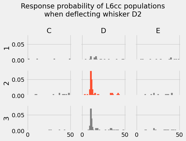
[26]:
ct = "L5tt"
whisker = "C2"
fig, axs = activity_gridplot(ct, deflected_whisker=whisker)
I.plt.show()
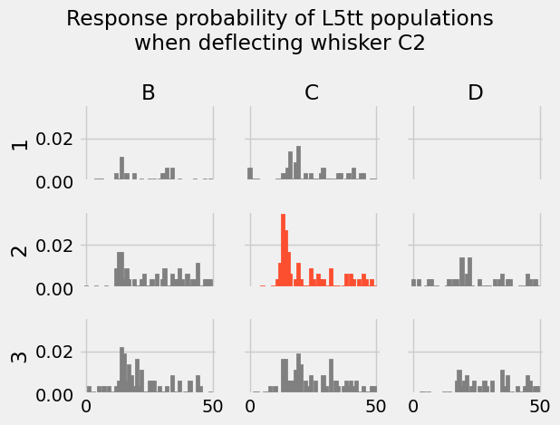
Recap
Tutorial 2.1 covered how to embed a neuron model into a network reconstruction, taking into account the relevant morphological, cellular and network properties. This tutorial covered how to generate synaptic activity. We are now ready to combine our biophysically detailed neuron model with this network model: see Tutorial 3.1.