Multi-scale modeling¶

Tutorial 1.3 covered how to generate biophysically detailed compartmental models of a neuron. Tutorial 2.1 and Tutorial 2.2 covered how to embed neuron models into a network reconstruction, and how to generate synaptic activity that reflects an in vivo condition.

This tutorial will show how to combine the two models into a single multi-scale simlation.

[1]:

from pathlib import Path
tutorial_output_dir = f"{Path.home()}/isf_tutorial_output"  # <-- Change this to your desired output directory

[2]:

import Interface as I
from getting_started import getting_started_dir
db = I.DataBase(tutorial_output_dir)['network_modeling']

if not 'biophysical_constraints' in db.keys():
    cell_parameter_file = I.os.path.join(
        getting_started_dir,
        'example_data',
        'biophysical_constraints',
        '86_C2_center.param')
    I.shutil.copy(cell_parameter_file, db.create_managed_folder('biophysical_constraints'))
cell_parameter_file = db['biophysical_constraints'].join('86_C2_center.param')

[INFO] ISF: Current version: heads/docs+0.g1456ee0eb.dirty
[INFO] ISF: Current pid: 180678

Warning: no DISPLAY environment variable.
--No graphics will be displayed.

[INFO] l5pt: Loaded mechanisms in NEURON namespace.
[ATTENTION] ISF: The source folder has uncommited changes!



[INFO] ISF: Loaded modules with __version__ attribute are:
IPython: 8.12.2, Interface: heads/docs+0.g1456ee0eb.dirty, PIL: 9.4.0, _brotli: 1.0.9, _csv: 1.0, _ctypes: 1.1.0, _curses: b'2.2', _decimal: 1.70, argparse: 1.1, backcall: 0.2.0, blosc: 1.11.1, bluepyopt: 1.9.126, brotli: 1.0.9, certifi: 2024.08.30, cffi: 1.17.0, charset_normalizer: 3.4.0, click: 7.1.2, cloudpickle: 3.1.0, colorama: 0.4.6, comm: 0.2.2, csv: 1.0, ctypes: 1.1.0, cycler: 0.12.1, cytoolz: 0.12.3, dash: 2.18.2, dask: 2.30.0, dateutil: 2.9.0, deap: 1.4, debugpy: 1.8.5, decimal: 1.70, decorator: 5.1.1, defusedxml: 0.7.1, distributed: 2.30.0, distutils: 3.8.15, entrypoints: 0.4, executing: 2.1.0, fasteners: 0.17.3, flask: 1.1.4, fsspec: 2024.10.0, future: 1.0.0, greenlet: 3.1.1, idna: 3.10, ipaddress: 1.0, ipykernel: 6.29.5, ipywidgets: 8.1.5, isf_pandas_msgpack: 0.4.0, itsdangerous: 1.1.0, jedi: 0.19.1, jinja2: 2.11.3, joblib: 1.4.2, json: 2.0.9, jupyter_client: 7.3.4, jupyter_core: 5.7.2, kiwisolver: 1.4.5, logging: 0.5.1.2, markupsafe: 2.0.1, matplotlib: 3.5.1, msgpack: 1.0.8, neuron: 7.8.2+, numcodecs: 0.12.1, numexpr: 2.8.6, numpy: 1.19.2, packaging: 25.0, pandas: 1.1.3, parso: 0.8.4, past: 1.0.0, pexpect: 4.9.0, pickleshare: 0.7.5, platform: 1.0.8, platformdirs: 4.3.6, plotly: 5.24.1, prompt_toolkit: 3.0.48, psutil: 6.0.0, ptyprocess: 0.7.0, pure_eval: 0.2.3, pydevd: 2.9.5, pygments: 2.18.0, pyparsing: 3.1.4, pytz: 2024.2, re: 2.2.1, requests: 2.32.3, scipy: 1.5.2, seaborn: 0.12.2, six: 1.16.0, sklearn: 0.23.2, socketserver: 0.4, socks: 1.7.1, sortedcontainers: 2.4.0, stack_data: 0.6.2, statsmodels: 0.13.2, tables: 3.8.0, tblib: 3.0.0, tlz: 0.12.3, toolz: 1.0.0, tqdm: 4.67.1, traitlets: 5.14.3, urllib3: 2.2.3, wcwidth: 0.2.13, werkzeug: 1.0.1, yaml: 6.0.2, zarr: 2.15.0, zlib: 1.0, zmq: 26.2.0, zstandard: 0.19.0

Simulating synaptic activity¶

The previous tutorials on network modeling provided us with a functional network that mimics the in vivo condition of the passive touch of a whisker.

Here, we will simulate multiple trials for one single whisker stimulus, and save the result in the database under the simrun key.

[76]:

# Delete previous results, if they exist
if 'simrun' in db.keys():
    del db['simrun']

# Create new folder for results
db.create_managed_folder('simrun')

[WARNING] isf_data_base: ISF has uncommitted changes - reproducing results may not be possible.

[76]:

'/gpfs/soma_fs/home/meulemeester/isf_tutorial_output/network_modeling/db/simrun'

Let’s simulate \(4\) trials on each of \(4\) workers, resulting in \(16\) trials total. These trials all use the same neuron and network parameters, but contain stochasticity in:

• The activation probability for each presynaptic cell (based on population-specific PSTHs)

• The activation probability for each synapse, as captured by the releaseProb parameter in the Network parameters

The locations of these synapses is deterministically captured by the .syn files referenced in the Network parameters. If you want to explore different possible synapse locations, you should create multiple embeddings (see Tutorial 2.1) and from there also create multiple Network parameter files.

[89]:

stimulated_whisker = "C2"  # Primary whisker: cell is also in the C2 column

network_file = db['network_param'].join('{}_stim.param'.format(stimulated_whisker))
dir_prefix = db['simrun'].join('stim_{}'.format(stimulated_whisker))

nSweeps = 4     # number of consecutive simulations per task
nprocs = 4      # number of processes simulating that task in parallel
tStop = 300     # stop the simulation at t=300ms (make sure this is later than the stimulus onset = 245ms)

d = I.simrun_run_new_simulations(
    cell_parameter_file, # defined in the above cell
    network_file,
    dirPrefix = dir_prefix,
    nSweeps = nSweeps,
    nprocs = nprocs,
    tStop = tStop,
    silent = False)

I.simrun_run_new_simulations returns dask.delayed objects. These describe how the computation can be run, but it is not computed yet. We send it to our distributed cluster for that:

[78]:

client = I.get_client()
futures = client.compute(d)

AS usual, you can inspect the progress on the dashboard:

[74]:

client

[74]:

[79]:

from dask.distributed import wait
wait(futures)

[79]:

DoneAndNotDoneFutures(done={<Future: finished, type: builtins.str, key: lambda-2ad8a915-d4c2-4125-a619-6a9ee5e01d3c>, <Future: finished, type: builtins.str, key: lambda-401d929f-3cba-4b03-a65b-890ad6e6fd06>, <Future: finished, type: builtins.str, key: lambda-99d7c556-de05-4ebe-a71a-c7599c6a636e>, <Future: finished, type: builtins.str, key: lambda-f3ec2c52-e69b-4879-9b23-593f67516b69>}, not_done=set())

After this is complete, the “simrun” folder in the DataBase contains the simulation results

[80]:

db['simrun'].listdir()

[80]:

['Loader.json', 'metadata.json', 'stim_C2']

Analyzing the results¶

here, we use DataBase to parse our simulation results to high-performance file formats. For more info, refer to the data_base.db_initializers. These initialize simulation results in a database for convenient access to the data using the widely used pandas and dask libraries. It also converts the data to an optimized binary format: msgpack. This gives the following advantages:

• the msgpack format is extremely fast

• msgpack allows for blosc compression, reducing space on hard drive (<25% of original data)

• cell activation data is categorized i.e. repeated values are replaced by an integer

[81]:

I.db_init_simrun_general.init(
    db,
    db['simrun'],
    client=client
)

[WARNING] isf_data_base: ISF has uncommitted changes - reproducing results may not be possible.
[WARNING] isf_data_base: ISF has uncommitted changes - reproducing results may not be possible.

Now, the following keys are set:

Let’s have a look at the synapse activation data frame:

[82]:

db['synapse_activation']

[82]:

This is a dask dataframe object. Instead of loading the data fully, it is a pointer to the actual data. Only when actual computations need to be done, are the values of the data loaded. Until then, it will only provide relevant metadata. Let’s explicitly load a small fraction of the data to have a look:

[83]:

head = db['synapse_activation'].head(2)
head

[83]:

We can see that the dataframe saves each synapse activation, including the synapse type, where on the neuron this synapse was (both in terms of soma distance, and section ID). The activation times are saved in the numbered clumns on the right. It is possible for a synapse to activate more than once during a simulation, which is why there are multiple numbered columns.

We can select data using the sim_trial_index as well, which indexes all synapse activations that belong to a single simulation:

[84]:

some_index = db['synapse_activation'].compute().index[0]
db['synapse_activation'].loc[some_index]

[84]:

This returns a dask dataframe again; the query is not computed yet. To do this, call compute:

[85]:

db['synapse_activation'].loc[some_index].compute()

[85]:

Let’s put our dask knowledge to use: what is the average distance of synapses from the soma by celltype? WE can calculate this efficiently by mapping function to each dask partition:

[86]:

# load dask dataframe
sa = db['synapse_activation']
# assign a new column: the celltype is the first part of the synapse_type column
sa['celltype'] = sa.map_partitions(lambda x: x.synapse_type.str.split('_').str[0])
# groupb by this value, compute the mean soma distance in each group, compute the result on the cluster
sa.groupby('celltype').apply(lambda x: x.soma_distance.mean()).compute(scheduler=client)

[WARNING] py: `meta` is not specified, inferred from partial data. Please provide `meta` if the result is unexpected.
  Before: .apply(func)
  After:  .apply(func, meta={'x': 'f8', 'y': 'f8'}) for dataframe result
  or:     .apply(func, meta=('x', 'f8'))            for series result

[86]:

celltype
SymLocal5     102.895287
SymLocal6      69.224869
VPM           283.171998
L4ss          384.213487
L34           472.821345
L5st          763.656384
SymLocal2     523.960223
L45Sym        235.565295
L56Trans      155.026705
L45Peak       370.852195
L4sp          499.375684
L2            730.177047
L4py          290.263935
L6cc          324.280091
L5tt          227.409182
SymLocal1    1159.022063
SymLocal4     129.119649
L23Trans      979.915281
SymLocal3     211.627990
L6ccinv       239.657659
L6ct          176.161688
L1           1394.774783
dtype: float64

Visualization¶

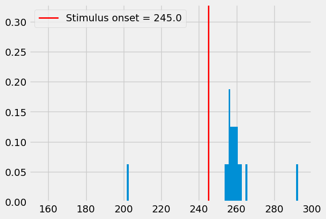
You can plot a PSTH of the response probabilities of these neurons to their synaptic input

[87]:

# Let's fetch the stimulus onset for visualization purposes:
example_ind = 0
example_population = "L6cc_C2"
netp_fn = db['parameterfiles'].iloc[example_ind]['path_network']
netp = I.scp.build_parameters(netp_fn)
stim_onset = netp.network[example_population].celltype.pointcell.offset

Note: different simulation trials and/or populations can in principle have different offset. That would mean that their PSTHs of evoked activity would have different beginnings relative to the simulation start. In this case however, we only consider a single stimulus for every trial and population, and so they all have the same offset. In other words, it does not matter here which population or simulation trial you check to fetch the offset.

Note: The cell models are initialized with default values, which are unlikely to be stable dynamical states. After \(\sim 100 - 200ms\), the models are usually stable. Activity during this period is simply due to stabilizin models, but has no explicit biological meaning.

[ ]:

%matplotlib inline
I.plt.style.use("fivethirtyeight")

converge_t = 150    # rough estimate on how slow models converge to rest state

fig = I.plt.figure()
bins, freqs = I.temporal_binning(db['spike_times'])
# Plot existing bins and values
I.plt.hist(bins[:-1], bins, weights = freqs)
I.plt.axvline(stim_onset, c='red', lw=2, label=f"Stimulus onset = {stim_onset}")
I.plt.xlim((converge_t, tStop))
I.plt.legend()
I.plt.show()

2D animation of membrane voltage¶

It is easy to create an animation of a simulation trial from the database:

[14]:

cell = I.simrun_simtrial_to_cell_object(db, some_index)

[15]:

if not 'D3_stim_animation' in db.keys():
    I.cell_to_animation(
        cell,
        xlim = [0,1500],
        ylim = [-90, 50],
        tstart = 245-25,
        tend = 245+25,
        tstep = 0.2,
        outdir = db.create_managed_folder('D3_stim_animation'))
I.display_animation(db['D3_stim_animation'].join('*', '*png'), embedded = True)

[WARNING] isf_data_base: ISF has uncommitted changes - reproducing results may not be possible.

– +

Once Loop Reflect

3D animation of the membrane voltage and synapse activations¶

[16]:

from visualize.cell_morphology_visualizer import CellMorphologyVisualizer

# # To remake the visualization, uncomment this code
# if I.os.path.exists(db._basedir/'D3_stim_animation_3d'):
#     I.shutil.rmtree(db._basedir/'D3_stim_animation_3d')

images_path = str(db._basedir/'D3_stim_animation_3d')

cmv = CellMorphologyVisualizer(
    cell,
    t_start=245-25,
    t_stop=245+25,
    t_step=0.2
    )

cell_population = cell.synapses.keys()
cell_population_colors = {
    synapse: I.plt.cm.Set3(i/len(cell_population))
    for i, synapse in enumerate(cell_population)}
cell_population_colors['inactive'] = "#f0f0f0"
cmv.population_to_color_dict = cell_population_colors

cmv.animation(
    images_path=images_path,
    color="voltage",
    show_synapses=True,
    client=I.get_client(),
)

– +

Once Loop Reflect

3D visualization of the membrane voltage and presynaptic cell activations¶

You can even visualize the soma locations of the active presynaptic cells.

As this requires 3D rendering, we are going to step out of python to visualize this. You can write out the postsynaptic cell and presynaptic locations as .vtk files: free, open-source and standardized. These can in principle be visualized in Python, but the rendering setup is a bit tedious. You can also use any rendering program that supports .vtk. We recommend Paraview.

[17]:

if not 'synapse_activation_vtk' in db.keys():
    db.create_managed_folder('synapse_activation_vtk')
db.ls()

<data_base.isf_data_base.isf_data_base.ISFDataBase object at 0x2b0fa5391a30>
Located at /gpfs/soma_fs/home/meulemeester/isf_tutorial_output/network_modeling/db
db
├── cell_activation
├── voltage_traces
├── simresult_path
├── metadata
├── anatomical_constraints
├── parameterfiles
├── synapse_activation_vtk
├── filelist
├── spike_times
├── D3_stim_animation
├── simrun
├── dendritic_spike_times
│   └── apical_proximal_distal_rec_sites_ID_000_sec_038_seg_032_x_0.929_somaDist_920.7_-30.0
├── dendritic_recordings
│   └── apical_proximal_distal_rec_sites_ID_000_sec_038_seg_032_x_0.929_somaDist_920.7
├── synapse_activation
├── parameterfiles_network_folder
├── biophysical_constraints
├── D3_stim_animation_3d
├── sim_trial_index
... (2 more)

Let’s map the presynaptic cells to their corresponding location. The activation of presynaptic cells, including their celltype, is given in the DataBase key "cell_acativation". Their locations are saved in the "anatomical_constraints" key.

[18]:

from simrun.utils import get_fraction_of_landmarkAscii_dir
soma_location_pdf = get_fraction_of_landmarkAscii_dir(1, db._basedir/'anatomical_constraints'/'presynaptic_somata')
ca = db['cell_activation'].loc[some_index].compute()
ca['celltype'] = [e.split("_")[0] for e in ca['presynaptic_cell_type']]
soma_location_pdf['celltype'] = [e.split("_")[-1] for e in soma_location_pdf['label']]

soma_location_pdf

[18]:

[19]:

outdir = I.os.path.join(db.basedir, 'synapse_activation_vtk')

cmv_unaligned = CellMorphologyVisualizer(
    cell,
    align_trunk=False,
    t_start=245-25,
    t_stop=245+25,
    t_step=0.2,
    )

cmv_unaligned.write_vtk_frames(
    I.os.path.join(outdir, 'cell_D3_stim.vtk'),
    color="voltage",
    client=I.get_client()
)

[20]:

from visualize.vtk import save_cells_landmark_files_vtk

outdir = db._basedir/'synapse_activation_vtk'
I.logger.setLevel("INFO")  # some more output
a = save_cells_landmark_files_vtk(
    ca,
    soma_location_pdf,
    times_to_show=cmv_unaligned.times_to_show,  # be sure the times are aligned
    outdir=outdir,
    tspan=5,  # amount of time the synapse stays visible after it has been activated
    set_index = ['celltype', 'cell_ID'])

[INFO] vtk: Celltype nr mapper: {'L1': 0, 'L23Trans': 1, 'L2': 2, 'L34': 3, 'L45Peak': 4, 'L45Sym': 5, 'L4py': 6, 'L4sp': 7, 'L4ss': 8, 'L56Trans': 9, 'L5st': 10, 'L5tt': 11, 'L6cc': 12, 'L6ccinv': 13, 'L6ct': 14, 'SymLocal1': 15, 'SymLocal2': 16, 'SymLocal3': 17, 'SymLocal4': 18, 'SymLocal5': 19, 'SymLocal6': 20, 'VPM': 21}
[WARNING] vtk: No celltypes passed. Using all celltypes in the dataset.

You can now inspect these files in a .vtk compatible program. The result should look like this: